12. LLM Finetuning

12.1. Motivation and Overview

Although a pretrained LLM (e.g., GPT-3) can already perform multitask, including reasoning, via prompting (e.g., few-shot prompting and CoT prompting), further finetuning can usually better adapt to downstream applications (including better following prompt instruction). Particularly for LLMs on the smaller end (<10B), prompt iteration can usually only achieve limited performance gain, finetuning is a much more efficient way to improve model performance with small amount of training data. Fundamentally, this is because the generic pretraining objective (predicting the next token) does not fully align with the downstream application objective: following instructions and conducting specific tasks.

This chapter explores two primary approaches to LLM finetuning: Instruction Finetuning and Parameter-Efficient Fine Tuning (PEFT). Instruction Finetuning focuses on teaching the model to follow specific instructions or prompts, enhancing its ability to understand instruction and reponse to instructions. PEFT techniques, on the other hand, aiming to finetune the model by updating only a small subset of its parameters, offering a more computationally efficient approach to customization.

12.2. Instruction Finetuning

12.2.1. Basics

Instruction finetuning [LZY24] for LLMs was developed to address the gap between the general knowledge and capabilities of pre-trained base models and the specific tasks or behaviors desired in real-world applications. While pre-trained LLMs possess broad knowledge, they often lack the ability to follow specific instructions or perform targeted tasks consistently.

As shown in the following example, a base LLM (without insturction finetuning) often fails to understand the intent of the prompt, and instead blindly performs text generation. An instructed LLM, on the other hand, understands the intent and provides useful responses.

Example 12.1 (Comparision of base LLM and instructed LLM in response to a prompt)

Given the prompt:

Task: Answer the following question about basic car maintenance concisely and accurately. Question: How often should you change your car’s oil, and why is it important?

Response from a base LLM (Qwen2.5-72B): Task: Provide a brief history of video games, including the evolution of game consoles and popular games. Question: How have video games and the gaming industry evolved over time? …

Response from an instruction-finetuned LLM (Qwen2.5-72B-instructed): You should change your car’s oil every 5,000 to 7,500 miles, or as recommended by your vehicle’s manufacturer. Regular oil changes are crucial because they remove contaminants that can damage engine components, ensuring the engine runs smoothly and efficiently, and extending its life.

The core idea of instruction finetuning [Fig. 12.1] is to train the model on a diverse set of task descriptions and their corresponding desired outputs. This typically involves:

1. Creating a dataset of instruction-output pairs covering a wide range of tasks.

2. Fine-tuning the pre-trained LLM on this dataset, often using supervised learning techniques.

Instruction tuning can often substantially improves zero shot performance on unseen tasks [WBZ+21].

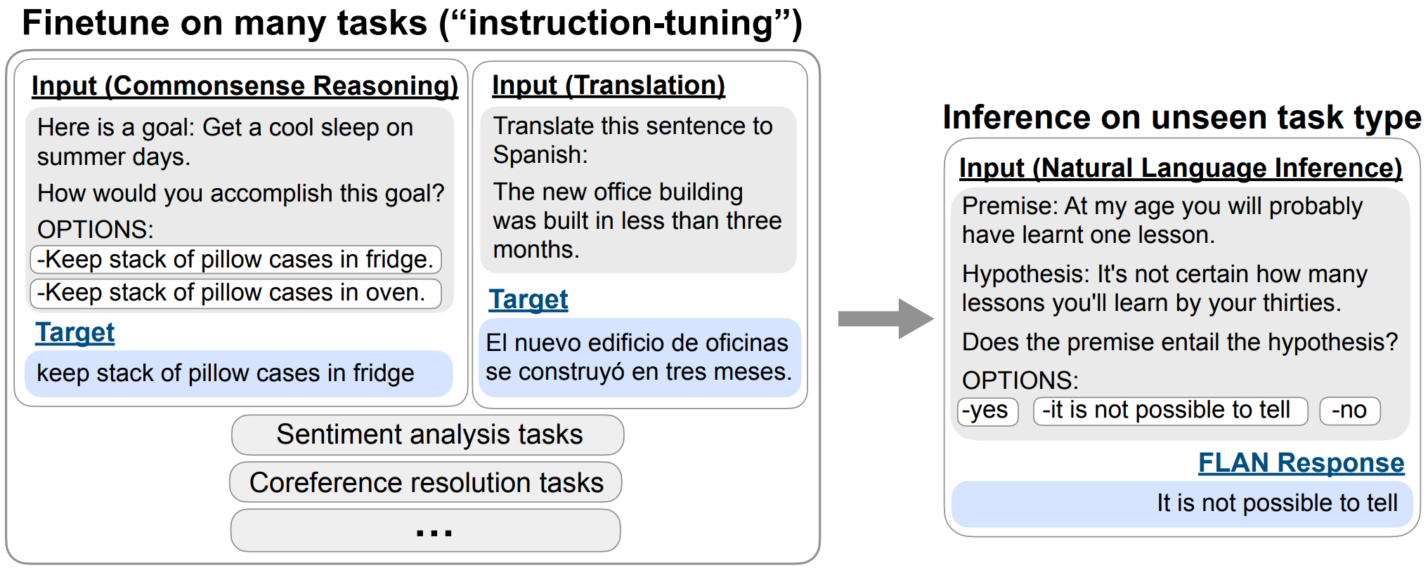
Fig. 12.1 Overview of instruction tuning and FLAN. Instruction tuning finetunes a pretrained language model on a mixture of tasks phrased as instructions. At inference time, we evaluate on an unseen task type; for instance, we could evaluate the model on natural language inference (NLI) when no NLI tasks were seen during instruction tuning. Image from [CHL+22]

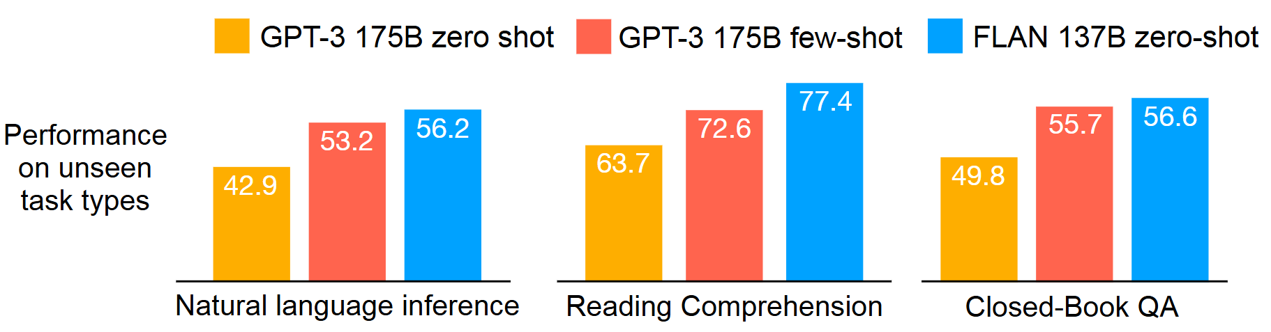
Fig. 12.2 Performance of zero-shot FLAN, compared with zero-shot and few-shot GPT-3, on three unseen task types where instruction tuning improved performance substantially. Image from [WBZ+21].

The following summarize the Pros and Cons of instruction finetuning.

Pros

• Improved multi-task performance: Instruction-tuned models can better understand and execute specific tasks, thus directly unlocking the multi-task ability of base model without task-specific prompting and fine-tuning.

• Better alignment with human intent and expectation: Models become more adept at interpreting and following natural language instructions as well as generating human expected results. Properly instruction-tuned models may be less likely to produce harmful or undesired content.

Cons

• Potential for overfitting: As it is usually difficult to creating diverse and high-quality instruction datasets, the model might overfit to the specific instructions in the training set. Ensuring comprehensive coverage of possible tasks and instructions is critical but challenging.

• Bias and compromising existing general knowledge: Aggressive instruction tuning might cause the model to forget some of its pre-trained knowledge. The instruction dataset may inadvertently introduce new biases into the model.

• Increased training costs: Additional fine-tuning requires computational resources and time.

12.2.2. Insturction Finetuning Loss Functions

Typical instruction finetuning follows the idea of autoregressive language modeling and optimize the prediction over the completion tokens given the instruction.

Specifically, each input is a concatenation of an instruction \(X\) and a completion \(Y\). Let \(X\) be the instruction sequence \(\left\{x_1, x_2, \ldots, x_m\right\}\) and \(Y\) be the completion (output) sequence \(\left\{y_1, y_2, \ldots, y_n\right\}\). The model is optimized to predict each token in \(Y\) given all the previous tokens in \(X\) and \(Y\) up to that point:

\[ P\left(y_1, y_2, \ldots, y_n \mid x_1, x_2, \ldots, x_m\right)=\prod_{j=1}^n P\left(y_j \mid x_1, x_2, \ldots, x_m, y_1, y_2, \ldots, y_{j-1}\right) \]

The loss function, \(\mathcal{L}\) is given as as follows:

\[ \mathcal{L}=-\log P\left(y_1, y_2, \ldots, y_n \mid x_1, x_2, \ldots, x_m\right)=-\sum_{j=1}^n \log P\left(y_j \mid x_1, x_2, \ldots, x_m, y_1, y_2, \ldots, y_{j-1}\right). \]

Recent studies [SYW+24] also show that conducting language modeling on the instruction part, known as instruction modeling, can further help for scenarios like:

• The ratio between instruction length and output length in the training data is large

• Only a small amount of training examples are used for instruction tuning.

Intuitively, under instruction modeling, interactions related to instructions can be better adapted to achieve better prediction on the desired output. However, there are also hypotheses that instruction modeling can lead to overfitting.

12.2.3. Comparison with other approaches

Instruction tuning represents a middle ground between the traditional pretrain-finetune paradigm and the prompting paradigm in making LLM useful for a broad range of downstream tasks[Fig. 12.3].

The pretrain-finetune approach typically involves further training a pretrained model on task-specific datasets, which can be effective but often requires separate models and training for each task. Practically, this imposes maintainentce cost for many models and incurs costs for tackling new downstream tasks.

The prompting paradigm leverages the pretrained model’s knowledge through carefully crafted prompts, enabling zero-shot and few-shot learning but potentially suffering from inconsistent performance and prompt sensitivity.

Instruction tuning bridges these approaches by fine-tuning the model on a diverse set of instructions and tasks, aiming to create a single model capable of following natural language instructions across various domains. This method retains much of the flexibility and generalization capability of prompting while providing more consistent and reliable performance like task-specific fine-tuning. As a result, instruction-tuned models can often handle a wide array of downstream tasks without the need for task-specific models or extensive prompt engineering, offering a more versatile and user-friendly solution for deploying LLMs in real-world applications.

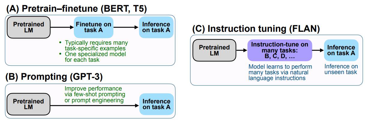
Fig. 12.3 Comparing instruction tuning with pretrain–finetune and prompting. Image from [WBZ+21].

12.2.4. Scaling Instruction Finetuning

Instruction Finetuning LLM can improve model performance and generalization to unseen tasks. In [CHL+22], scaling instruction finetuning over the number of tasks and model sizes are explored.

The key methodological aspects of the study are:

• Instruction finetuned LLMs on a diverse set of language tasks (up to 1,836 ). Training data is constructed as mixtures of different number of tasks.

• The study scales up both model size and number of finetuning tasks

As shown in Fig. 12.4, the key findings are

• Instruction finetuning significantly improved performance across a range of evaluations, especially for zero-shot and few-shot tasks

• Scaling to larger models and more diverse finetuning tasks led to better performance

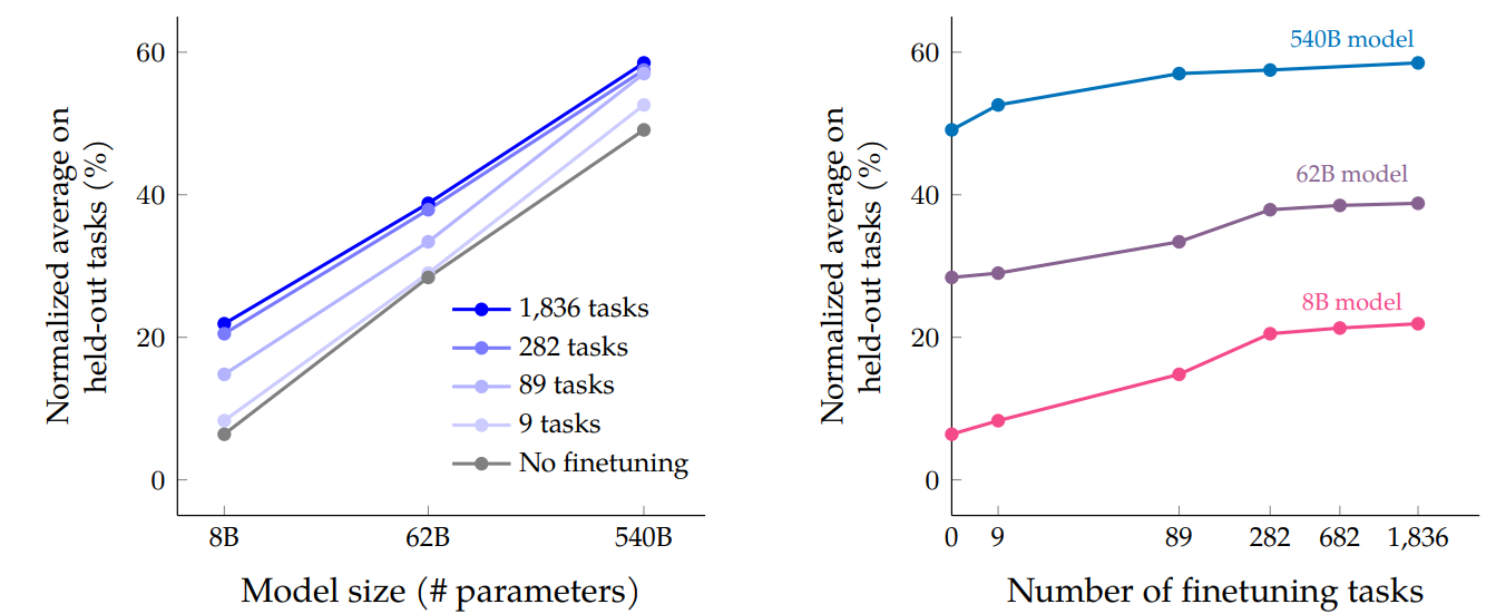
Fig. 12.4 Scaling behavior of multi-task instruction finetuning with respect to model size (# parameters) and number of finetuning tasks. Image from [CHL+22].

The study also explores the impact of inclusion/exclusion of CoT training data on reasoning tasks. One key observation [Fig. 12.5] is that instruction finetuning without CoT actually degrades reasoning ability. On the other hand, including just nine CoT datasets improves performance on all evaluations (including reasoning and non-reasoning tasks).

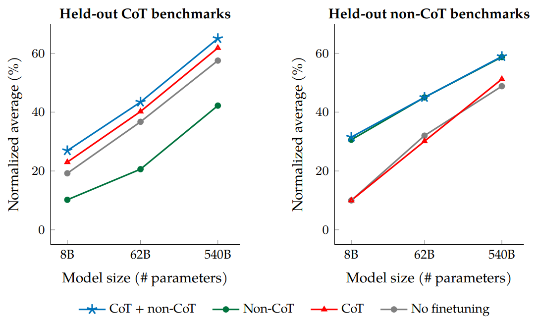
Fig. 12.5 Jointly finetuning on non-CoT and CoT data improves performance on both evaluations, compared to finetuning on just one or the other. Image from [CHL+22].

12.2.5. Bootstraping Instruction Finetuning

Given a base language that can mostly rely on few-shot prompting to complete tasks, we can further boostrap the model by

• Prompt the model to generate a diverse set of instruction-completion pair data from a limited set of seed task data.

• Fine-tuning the model on the self-generated training data.

This process is also known as Self-Instruct (Fig. 12.6), with the following key steps:

• The process starts with a small seed set of tasks as the task pool.

• Random tasks are sampled from the task pool, and used to prompt an off-the-shelf LM to generate both new instructions and corresponding completions.

• Filtering low-quality or similar generations, and then added back to the initial task pool.

To ensure that diverse instruction examples are generated, the filtering steps can use ROUGE-L similarity score to remove candidates that are similar to the any existing instructions.

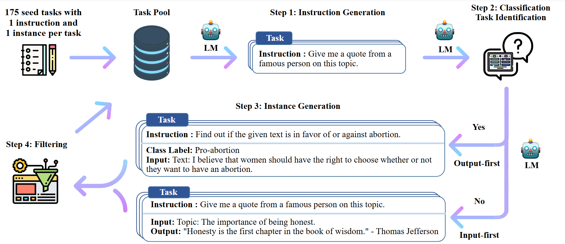
Fig. 12.6 A high-level overview of Self-Instruct. Image from [WWS+22].

As shown in the following table, Self-Instruct boosts the instruction-following ability of GPT3 by a large margin. The vanilla GPT3 model basically cannot follow human instructions at all. Notable, the self-instructed GPT3 nearly matches the performance of InstructGPT, which is trained with private user data and human-annotated labels.

Model	# Params	ROUGE-L
GPT3	175 B	6.8
GPT3 \(_{\text {Self-InsT }}\)	175 B	39.9
InstructGPT	175 B	40.8

12.3. Parameter-Efficient Fine Tuning (PEFT)

12.3.1. Motivation

To adapt a LLM to a specific downstream task, Full-size fine-tunning the whole LLM is usually not cost effective. For models whose model parameters are at the 1B or above, it is difficult to fine-tune the model using a single consumer grade GPU. Full-size finetuning also runs the risk of Catastrophic Forgetting [LYM+24] which means LLMs forget prior knowledge when learning new data.

Since the size of the fine-tuned dataset is typically much smaller than the pretrained dataset, performing full fine-tuning to update all the pretrained parameters may lead to overfitting.

PEFT [XXQ+23] emerges as a cost-effiective approach to LLM finetuning. In essence, PEFT only pdates only a small number of additional parameters or updates a subset of the pretrained parameters, preserving the knowledge captured by the PLM while adapting it to the target task and reducing the risk of catastrophic forgetting.

12.3.2. Adapter Tuning

The key idea of Adapter Tuning [HGJ+19] is to add several additional trainable modules (i.e., layers) to the Transformer that acting as adapting module and at the same time freeze the remaining model weights the original LLM. The intuition is that by these adapter modules can be trained to assist the original LLM to better adapt to downstream tasks.

As shown in Fig. 12.7, in each Transformer layer, adapter module are added at different places: after the multihead attention and after FFD. The output of the adapter is directly fed into the following layer normalization. The adaptor module can use a bottleneck architure to save compute cost. Specifically, The adapters first project the original \(d_{model}\)-dimensional features into a smaller dimension, \(m\), apply a nonlinearity, then project back to \(d_{model}\) dimensions.

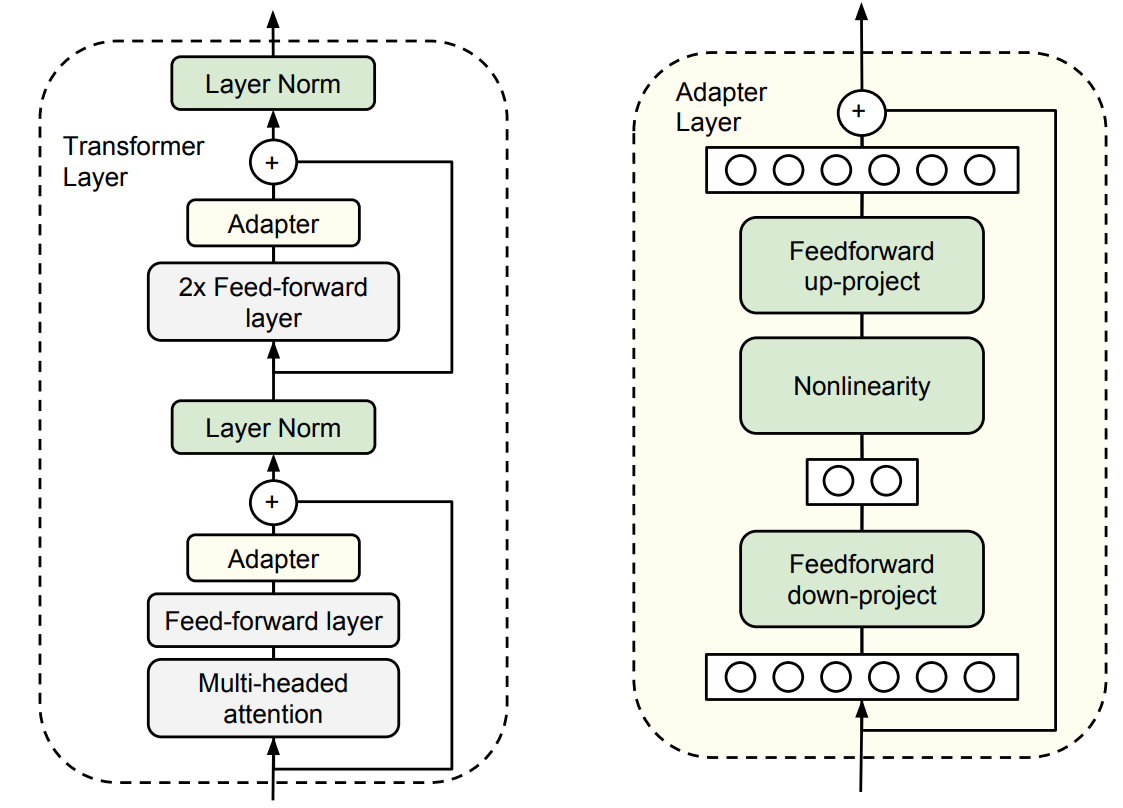
Fig. 12.7 Architecture of the adapter module and its integration with the Transformer. (Left) Adapter module are added at different places in each Transformer layer: after the projection following multihead attention and after the position-wise FFD layers. (Right) The adapter consists of a bottleneck first mapping the input to lower dimensions and then mappign the output to higher dimensions. Image from [HGJ+19].

12.3.3. Prompt Tuning

Prompt tuning [LARC21] is a technique that involves learning a small set of continuous task-specific vectors (soft prompts) while keeping the pretrained model parameters frozen. Specifically [Fig. 12.8], additional \(l\) learnable prompt token vectors, \(P=\left[P_1\right],\left[P_2\right], \cdots,\left[P_l\right]\), are combined with the model input \(X \in \mathbb{R}^{n \times d}\) to generate the final input \(\hat{X}\), that is,

\[\hat{X} = \operatorname{Concat}(P, X) = [P, X] \in \mathbb{R}^{(l+n)\times d}.\]

During fine-tuning, only the prompt token parameters of \(P\) are updated through gradient descent, while pretrained parameters remain frozen. When applying prompt tuning to the multi-task fine-tuning scenario, we can have task-specific prompt tokens work with a fixed pretrained model.

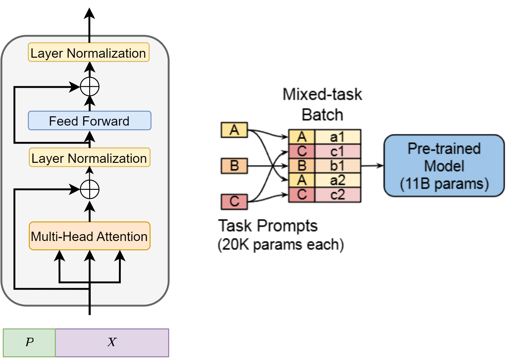
Fig. 12.8 Illustration of prompt tuning, where we concat a task-dependent prompt tokens into existing prompt

Studies [Fig. 12.9] show that using longer prompt length will achieve much better model performance than using single tuning prompt. One useful tuning prompt token initilization is class label initialization, where we used the the embeddings for the string representations of each class in the downstream task and use them to initialize one of the tokens in the prompt.

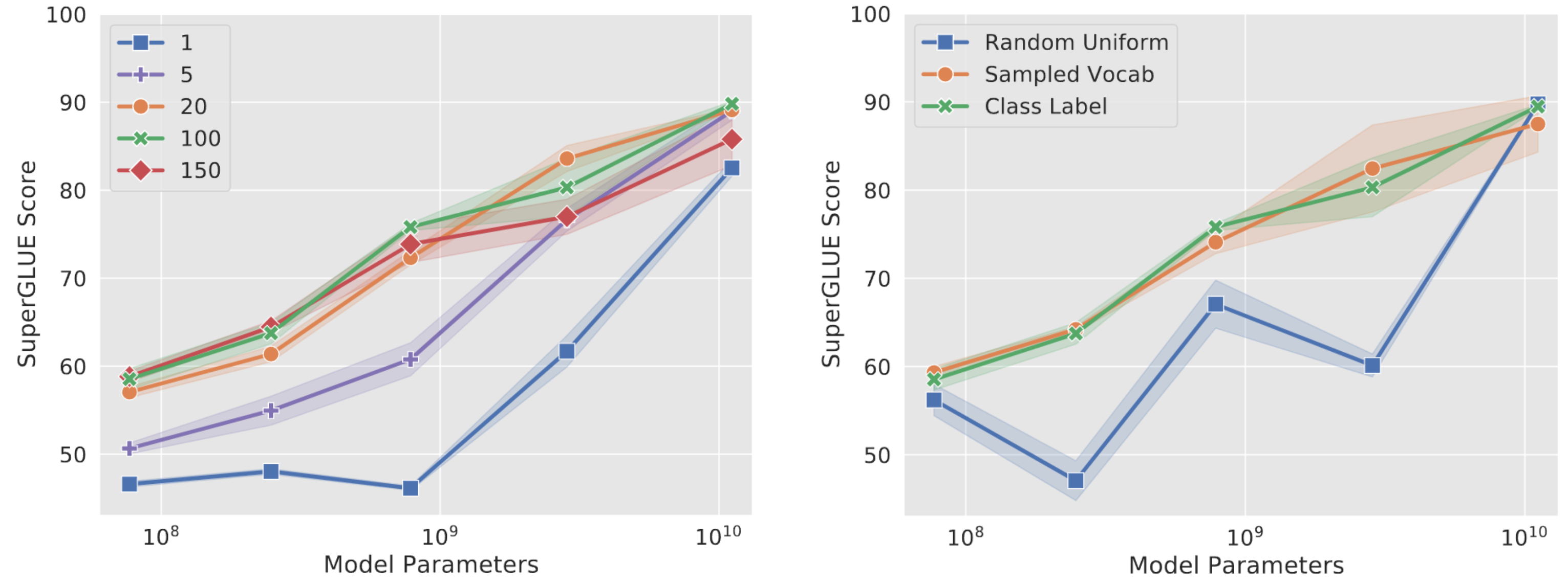
Fig. 12.9 Studies on the impact of length of prompt tuning tokens and its initialization.

12.3.4. Prefix-tuning

Prefix-tuning [LL21] proposes to prepend soft prompts \(P=\) \(\left[P_1\right],\left[P_2\right], \cdots,\left[P_l\right]\) ( \(l\) denotes the length of the prefix) to the hidden states of the multi-head attention layer, differing from prompt-tuning that adds soft prompts to the input. To ensure stable training, a FFN is introduced to parameterize the soft prompts, as direct optimization of the soft prompts can lead to instability. Two sets of prefix vectors \(\hat{P}_k\) and \(\hat{P}_v\) are concatenated to the original key \((K)\) and value \((V)\) vectors of the attention layer. The self-attention mechanism with prefix-tuning can be represented by Equation 8. During training, only \(\hat{P}_k, \hat{P}_v\), and the parameters of FFN are optimized, while all other parameters of PLMs remain frozen. The structure of prefix-tuning is illustrated in Fig. 12.10. After training, the FFN is discarded, and only \(P_k\) and \(P_v\) are used for inference.

\[ head=\operatorname{Attention}\left(X W_q,\operatorname{Concat}\left[\hat{P}_k, X W_k\right],\operatorname{Concat}\left[\hat{P}_v, X W_v\right]\right) \]

where \(\hat{P}_k=\operatorname{FFN}\left(P_k\right), \hat{P}_v=\operatorname{FFN}\left(P_v\right).\)

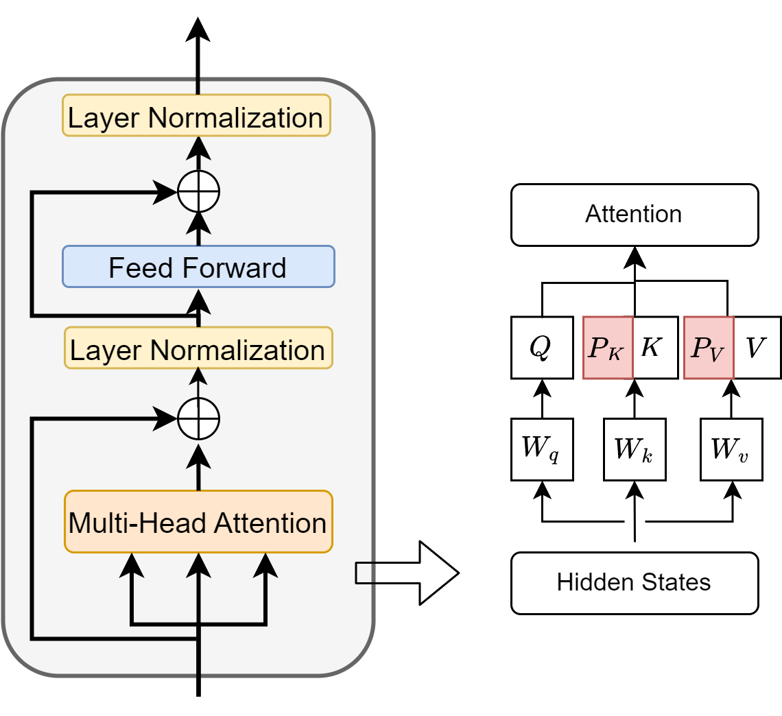
Fig. 12.10 Illustration of prefix tuning, where we concat task dependent prefix vectors into original \(K,V\) matrices.

12.3.5. LoRA (Low-Rank Adaptation)

12.3.5.1. The hypothesis and method

LoRA [HSW+21] is one of the most influential strategy among PEFT strategies. Compared with Adapter Tuning, which needs to add sequential layers vertically, and with Prompt Tuning,Prefix-tuning, which need to expand input vectors with extra tokens, LoRA is much more elegant approach from the perspective of archectural design and mathematics.

Use the notation that each downstream task is represented by a training dataset of input-target pairs: \(Z = \{(x_i, y_i), i=1,2,...,N\}\), where both \(x_i\) is the input prompt tokens, and \(y_i\) are response/completion tokens.

The key observation is that, we can express model fine-tuning on model weight \(\Phi\) in its full-update-formulation

\[ \max _{\Phi} \sum_{(x, y) \in \mathcal{Z}} \sum_{t=1}^{|y|} \log \left(P_{\Phi}\left(y_t \mid x, y_{<t}\right)\right) \]

as its incremental update form

\[ \max _{\theta} \sum_{(x, y) \in \mathcal{Z}} \sum_{t=1}^{|y|} \log \left(p_{\Phi_0+\Delta \Phi(\theta)}\left(y_t \mid x, y_{<t}\right)\right) \]

and make the assumption that task-specific parameter increment \(\Delta \Phi(\Theta)\) is further encoded by a much smaller-sized set of parameters \(\Theta\) with \(|\Theta| \ll\left|\Phi_0\right|\).

Specifically and as a further approximation, we only consider the LoRA on projeciton matrices \(W_Q, W_K, W_V\). Take \(W_Q\) as example.

\[H = XW^Q = X(W^{Q}_0 + \Delta W) = X(W^Q_0 + \underbrace{B^QA^Q}_{\text{Low Rank}}).\]

Here during finetuning, we freeze \(W^Q_0\) and update low rank matrices \(B^Q \in \mathbb{R}^{d_{model}\times r}\), \(A^Q \in \mathbb{R}^{r\times d_{head}}\), with \(r \ll \min(d_{model}, d_{head})\) (e.g., \(r <= 8\)).

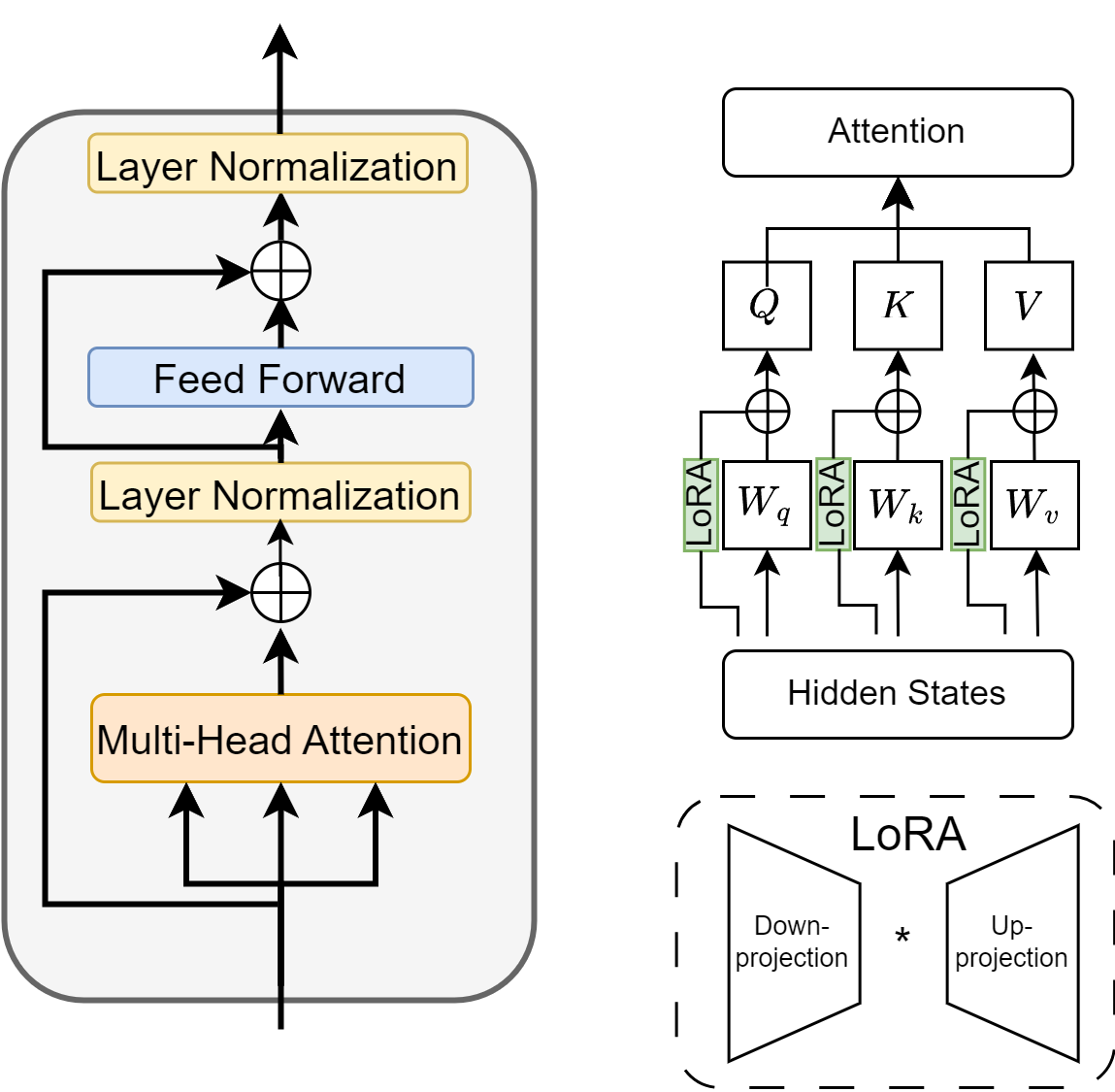
Fig. 12.11 Illustration of LoRA, where we provide low-rank matrix adapation on projection matrices in the attention layer.

Remark 12.1 (\(A,B\) initialization and model inference)

• To help stablize training, \(A,B\) is initialized in a way to ensure \(AB = 0\). Specifically, we can set one matrix (say \(A\)) to zero, and initialize \(B\) with random values. For \(AB\neq 0\), the initial training phase can be unstable due to large changes of model weights.

• After training, we only need to save low-rank matrices \(A\) and \(B\) for different tasks. During inference, we can add \(AB\) onto the original projection matrices. Unlike previous Adapter approach, there is no additional inference latency.

12.3.5.2. Study Results

As shown in the following, LoRA has been successfully applied to various models, including RoBERT and GPT-3, showing competitive performance with full finetuning while using only 0.01% of the trainable parameters.

Table 12.1 RoBERT with different adaptation methods on the language understanding GLUE benchmark.

Model & Method	# Trainable Parameters	Avg.
RoB_base (FT)	125.0M	86.4
RoB_base (Adpt^D)	0.9M	85.4
RoB_base (LoRA)	0.3M	87.2

Table 12.2 GPT-3-175B with different adaptation methods on the language understanding benchmark.

Model&Method	# Trainable Parameters	WikiSQL Acc. (%)	MNLI-m Acc. (%)	SAMSum R1/R2/RL
GPT-3 (FT)	\(175,255.8 \mathrm{M}\)	\(73.8\)	89.5	\(52.0 / 28.0 / 44.5\)
GPT-3 (Adapter )	40.1 M	73.2	91.5	\(53.2 / 29.0 / 45.1\)
GPT-3 (LoRA)	4.7 M	73.4	\(\mathbf{91.7}\)	53.8/29.8 /45.9
GPT-3 (LoRA)	37.7 M	\(\mathbf{7 4 . 0}\)	\(\mathbf{9 1 . 6}\)	\(53.4 / 29.2 / 45.1\)

The paper also studies the effect of low rank parameter \(r\) on model performance as well as adaptation choices on \(\left\{W^Q,W^K,W^V,W^O\right\}\),

As shown in the following table,

• \(r\) as small as one suffices for adapting both \(W^Q\) and \(W^V\) on these datasets while training \(W^Q\) alone needs a larger \(r\).

• Adapting more matrices will improve model performance but has marginal gain when adapting all matrices.

Table 12.3 Validation accuracy on WikiSQL and MultiNLI with different rank \(r\).

	Weight Type	\(r=1\)	\(r=2\)	\(r=4\)	\(r=8\)	\(r=64\)
WikiSQL	\(W^Q\)	68.8	69.6	70.5	70.4	70.0
	\(W^Q, W^V\)	73.4	73.3	73.7	73.8	73.5
	\(W^Q, W^K, W^V, W^O\)	74.1	73.7	74.0	74.0	73.9
MultiNLI	\(W^Q\)	90.7	90.9	91.1	90.7	90.7
	\(W^Q, W^V\)	91.3	91.4	91.3	91.6	91.4
	\(W^Q, W^K, W^V, W^O\)	91.2	91.7	91.7	91.5	91.4

12.4. Scaling Law for Fine Tuning

When adapting LLM to specific downstream tasks, there are two popular ways of finetuning: full-model tuning (FMT) that updates all LLM parameters and PEFT that only optimizes a small amount of (newly added) parameters, such as prompt tuning and LoRA.

It is an open question on how the resulting model performs with regards to fine-tuning data size, model size, and tuning parameter size (in the PEFT case)

[ZLCF24] proposes the following multiplicative joint scaling law for LLM finetuning:

\[ \hat{\mathcal{L}}\left(X, D_f\right)=A \times \frac{1}{X^\alpha} \times \frac{1}{D_f^\beta}+E, \]

where \(\{A, E, \alpha, \beta\}\) are data-specific parameters to be fitted, \(D_f\) denotes finetuning data size, and \(X\) refer to other scaling factors (like model size, and tuning parameter size) and \(L\) is perplexity. After fitting to scaling experiments, larger \(\alpha\) or \(\beta\) means the bigger contribution from these factors.

The key findings are

• Finetuning model performance scales better on model size than fine-tuning data size, as indicated by larger \(\alpha\) then \(\beta\) in Fig. 12.12,Fig. 12.13. This suggests that using a larger LLM model is preferred for finetuning over larger data.

• Finetuning data size have more pronounced influence on FMT than PET (much larger \(\beta\) in FMT), where LoRA scales better than Prompt. In other words, FMT is more data hungary and also benefits more from increasing finetuning data.

• Compared across different PEFT approach, scaling tuning parameters is ineffective, delivering limited gains for both LoRA and Prompt. At the end of day, the amount of newly added trainable parameters often forms a bottleneck for the expressivity of the model.

Fig. 12.12 Joint scaling law for model size (from 1B to 16B) and fine-tuning data sizes for translation task. Image from [ZLCF24].

Fig. 12.13 Joint scaling law for model size (from 1B to 16B) and fine-tuning data sizes for summarization task. Image from [ZLCF24].

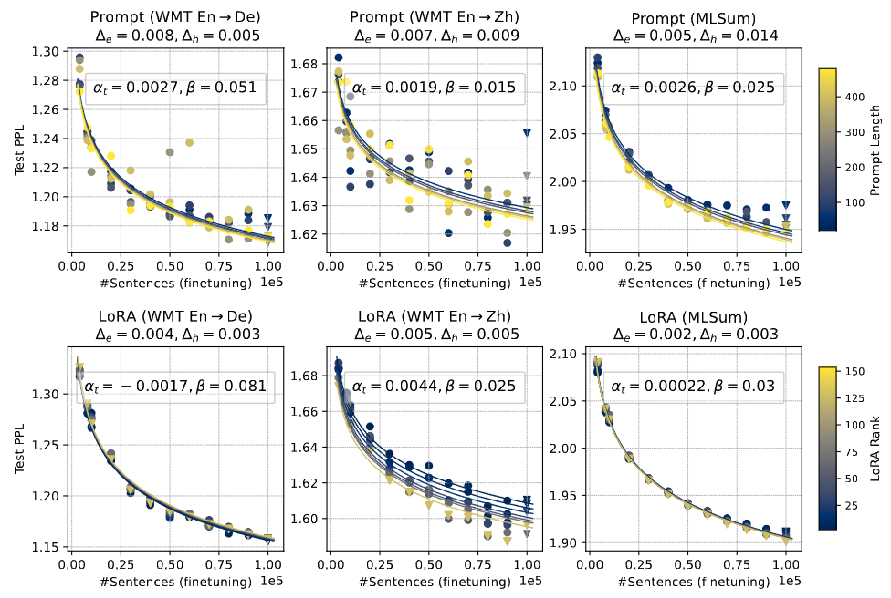
Fig. 12.14 Joint scaling law for tuning parameter size and fine-tuning data sizes for summarization task. Image from [ZLCF24].

12.5. Bibliography

[CHL+22] (1,2,3,4)

Hyung Won Chung, Le Hou, Shayne Longpre, Barret Zoph, Yi Tay, William Fedus, Yunxuan Li, Xuezhi Wang, Mostafa Dehghani, Siddhartha Brahma, Albert Webson, Shixiang Shane Gu, Zhuyun Dai, Mirac Suzgun, Xinyun Chen, Aakanksha Chowdhery, Alex Castro-Ros, Marie Pellat, Kevin Robinson, Dasha Valter, Sharan Narang, Gaurav Mishra, Adams Yu, Vincent Zhao, Yanping Huang, Andrew Dai, Hongkun Yu, Slav Petrov, Ed H. Chi, Jeff Dean, Jacob Devlin, Adam Roberts, Denny Zhou, Quoc V. Le, and Jason Wei. Scaling instruction-finetuned language models. 2022. URL: https://arxiv.org/abs/2210.11416, arXiv:2210.11416.

[HGJ+19] (1,2)

Neil Houlsby, Andrei Giurgiu, Stanislaw Jastrzebski, Bruna Morrone, Quentin de Laroussilhe, Andrea Gesmundo, Mona Attariyan, and Sylvain Gelly. Parameter-efficient transfer learning for nlp. 2019. URL: https://arxiv.org/abs/1902.00751, arXiv:1902.00751.

[HSW+21]

Edward J. Hu, Yelong Shen, Phillip Wallis, Zeyuan Allen-Zhu, Yuanzhi Li, Shean Wang, Lu Wang, and Weizhu Chen. Lora: low-rank adaptation of large language models. 2021. URL: https://arxiv.org/abs/2106.09685, arXiv:2106.09685.

[LARC21]

Brian Lester, Rami Al-Rfou, and Noah Constant. The power of scale for parameter-efficient prompt tuning. arXiv preprint arXiv:2104.08691, 2021.

[LL21]

Xiang Lisa Li and Percy Liang. Prefix-tuning: optimizing continuous prompts for generation. arXiv preprint arXiv:2101.00190, 2021.

[LZY24]

Renze Lou, Kai Zhang, and Wenpeng Yin. Large language model instruction following: a survey of progresses and challenges. Computational Linguistics, pages 1–10, 2024.

[LYM+24]

Yun Luo, Zhen Yang, Fandong Meng, Yafu Li, Jie Zhou, and Yue Zhang. An empirical study of catastrophic forgetting in large language models during continual fine-tuning. 2024. URL: https://arxiv.org/abs/2308.08747, arXiv:2308.08747.

[SYW+24]

Zhengyan Shi, Adam X Yang, Bin Wu, Laurence Aitchison, Emine Yilmaz, and Aldo Lipani. Instruction tuning with loss over instructions. arXiv preprint arXiv:2405.14394, 2024.

[WWS+22]

Xuezhi Wang, Jason Wei, Dale Schuurmans, Quoc Le, Ed Chi, Sharan Narang, Aakanksha Chowdhery, and Denny Zhou. Self-consistency improves chain of thought reasoning in language models. arXiv preprint arXiv:2203.11171, 2022.

[WBZ+21] (1,2,3)

Jason Wei, Maarten Bosma, Vincent Y Zhao, Kelvin Guu, Adams Wei Yu, Brian Lester, Nan Du, Andrew M Dai, and Quoc V Le. Finetuned language models are zero-shot learners. ArXiv:2109.01652, 2021.

[XXQ+23]

Lingling Xu, Haoran Xie, Si-Zhao Joe Qin, Xiaohui Tao, and Fu Lee Wang. Parameter-efficient fine-tuning methods for pretrained language models: a critical review and assessment. 2023. URL: https://arxiv.org/abs/2312.12148, arXiv:2312.12148.

[ZLCF24] (1,2,3,4)

Biao Zhang, Zhongtao Liu, Colin Cherry, and Orhan Firat. When scaling meets llm finetuning: the effect of data, model and finetuning method. arXiv preprint arXiv:2402.17193, 2024.