5. Transformers#
5.1. Pretrained Language Models#
Pretrained language models are a key technology in modern natural language processing (NLP) that leverages large scale of un-labelled text data and computational power to drastically improve language understanding and generation tasks.
At their core, pretrained language models are large neural networks that have been exposed to enormous amounts of text data – including millions of books, articles, and websites. Through this exposure, they learn to recognize patterns in language, grasp context, and even pick up on subtle nuances in meaning.
The key advantage of pretrained language model lies in the fact that it can be universally adapted (i.e., fine-tuning) to all sorts of specific tasks with a small amount of labeled data. As a comparison, training a task-specific model from scratch would require large amount of labeled data, which can be expensive to obtain.
Pretrained language models typically use neural network architectures designed to process sequential data like text. The most prominent architectures in recent years have been based on the Transformer model, but there have been other important designs as well.
The Transformer architecture, introduced in 2017, has become the foundation for most modern language models. It uses a mechanism called self-attention to process input sequences in parallel, allowing the model to effectively capture long-range dependencies in text.
BERT (Bidirectional Encoder Representations from Transformers): BERT uses the encoder portion of the Transformer. It’s bidirectional, meaning it looks at context from both sides of each word when processing text. This makes it particularly good at language understanding tasks like sentence classification and named entity recognition.
GPT (Generative Pre-trained Transformer): GPT models use the decoder portion of the Transformer. They process text from left to right, making them well-suited for text generation tasks. Each version (GPT, GPT-2, GPT-3, etc.) has scaled up in size and capability.
5.2. Transformers Anatomy#
5.2.1. Overall Architecture#
Since 2007, Transformer [VSP+17] has emerged as one of most successful architectures in tackling challenging seq2seq NLP tasks like machine translation, text summarization, etc.
Traditionally, seq2seq tasks heavily use RNN-based encoder-decoder architectures, plus attention mechanisms, to transform one sequence into another sequence. Transformer, on the other hand, does not rely on any recurrent structure and is able to process all tokens in a sequence at the same time. This enables computation efficiency optimization via parallel optimization and address long-range dependency, both of which mitigate the shortcomings of RNN-based encoder-decoder architectures.
On a high level, Transformer falls into the category of encoder-decoder architecture, where the encoder encodes an input token sequence into low-dimensional embeddings, and the decoder takes the embeddings as input, plus some additional prompts, outputs an output sequence probabilities. The position information among tokens, originally stored in recurrent network structure, is now provided through position encoding added at the entry point of the encoder and decoder modules.
Attention mechanisms are the most crucial components in the Transformer architecture to learn contextualized embeddings and overcome the limitation of recurrent neural network in learning long-term dependencies (e.g., seq2seq model with attention).
The encoder module on the left [Fig. 5.1] consists of blocks that are stacked on top of each other to obtain the embeddings that retain rich information in the input. Multi-head self-attentions are used in each block to enable the extraction of contextual information into the final embedding. Similarly, the decoder module on the right also consists of blocks that are stacked on top of each other to obtain the embeddings. Two different types of multi-head attentions are used in each docder block, one is self-attention to capture contextual information among output sequence and one is to encoder-decoder attention to capture the dynamic information between input and output sequence.
In the following, we will discuss each component of transformer architecture in detail.
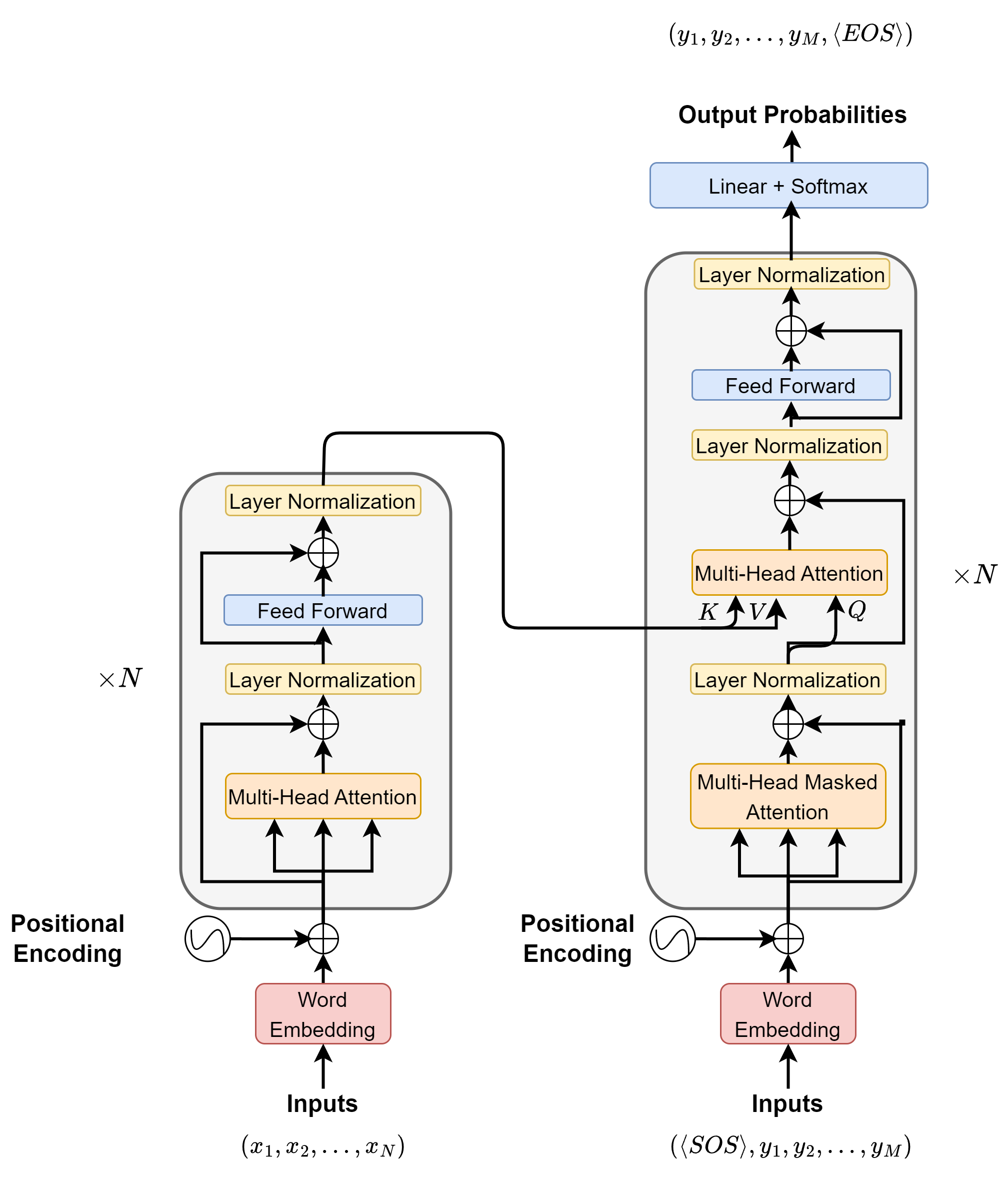
Fig. 5.1 The transformer architecture, which consists of an Encoder (left) and a Decoder (right).#
5.2.2. Input Output Conventions#
To understand the training and inference of transformer architecture, we need to distinguish different types of sequences:
Input sequence \(x = (x_1,x_2,...,x_p,..., x_n), x_i\in \mathbb{N}\) and input position sequence \(x^p = (1, 2, ..., n)\)
Output sequence \(y = (y_1,y_2,...,y_p,...,y_m), y_i \in \mathbb{N}\) and output position sequence \(y^p = (1, 2, ..., m)\). Output sequence is the input to the decoder.
Target sequence \(t = (t_1,t_2,...,t_p,...,t_m), t_i \in \mathbb{N}\). Input sequence and target sequence form a pair in the training examples.
For example, consider a translational task with input and target sequence given by Ich möchte eine Flasche Wasser and I want a bottle of water. In the typical supervised learning training, the input sequence, target sequence, and output sequence are in the following form
\(x = (Ich, möchte, eine, Flasche, Wasser, PAD, PAD)\)
\(t = (I, want, a, bottle, of, water, EOS, PAD)\)
\(y = (SOS, I, want, a, bottle, of, water, EOS)\)
The output sequence is the right-shifted target sequence with a starting token \code{SOS}. The output sequence will be fed into the decoder to predict the next token.
5.2.3. Position Encodings#
Consider an input sequence represented by an integer sequence \(x = (x_1,...,x_i,...,x_n), x_i\in \mathbb{N}\), \(e.g., x = (3, 5, 30, 2, ..., 21)\) that is fed into the Transformer architecture. For the input sequence \(s\), the word embedding vectors of dimensionality \(d_{model}\) alone do not encode positional information in the sequence. This can be fixed by utilizing a position encoding \(PE\) maps an integer index representing the position of the token in the sequence, \(x^p = (1, 2, ..., n)\) to \(n\) dense vectors with same dimensionality \(d_{model}\), i.e., \(\operatorname{PE}(s^p)\in \mathbb{R}^{n\times d_{model}}\).
The position encoding vectors can be specified in analytical forms and then be fixed during training. The position encoding mapping can also be learned from data. In theory, the specification of position encoding should preserve position information by mapping nearby positions to nearby high-dimensional vectors.
Notably, given the token position \(i \in \{1, ..., n\}\) \(\operatorname{PE}(i) \in \mathbb{R}^{d_{model}}\) is given by
where \(j = \{0,...,d_{model} - 1\}\). Note that the position encodings have the same dimension \(d_{model}\) as the word embeddings such that they can be summed. Intuitively, each dimension of the positional encoding corresponds to a sine/cosine wave of different wavelengths ranging from \(2 \pi\) (when \(j=1\)) to approx \(10000 \cdot 2 \pi\)(when \(j=d_{model}\)). An example position encodings of dimensionality 256 for position index from 1 to 256 is shown in Fig. 5.2.
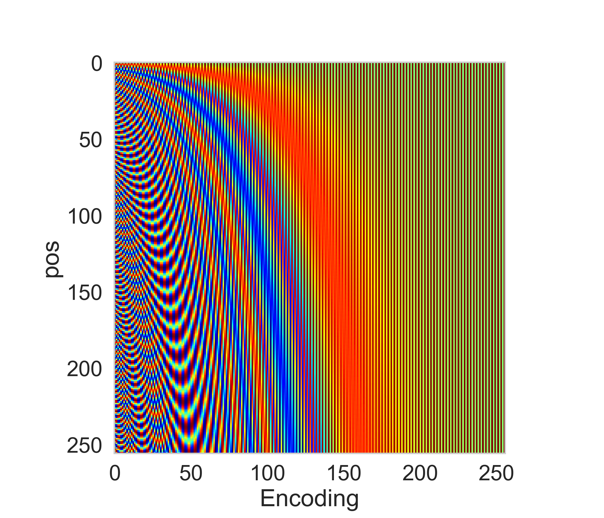
Fig. 5.2 Example position encodings of dimensionality 256 for position index from 1 to 256.#
Example 5.1
Let \(d_{model} = 2\), we have
Let \(d_{model} = 4\), we have
where \(w_0 = 1, w_1 = 1/10000^{2/4}\).
5.2.4. Multihead Attention with Masks#
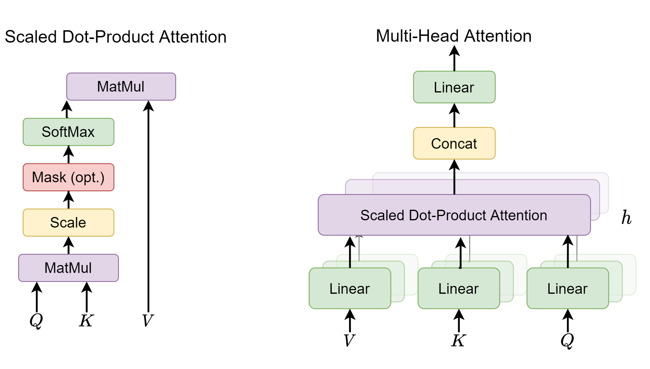
Fig. 5.3 The multi-head attention architecture.#
Multi-head attention mechanism with masks plays a central role in both encoder and decoder side. Attention mechanism enables contexualization and masks control the context each token can get access to. Attention of multiple heads, rather than a single head, allows the model to jointly attend to information from different representation subspaces at different positions [LTY+18].
Multi-head attentions are used in three places:
In the encoder module, multi-head attention without using masks are used to construct intermediate contextualized embedding for each token that depends of its context. The query, key, and values are all the same input sequence.
In the decoder module, multi-head attention with masks are used to construct contextualized embedding for each token by attending to only its preceding or seen tokens. The query, key, and values are all the same input sequence.
From the encoder module to the decoder module, multi-head attention without using masks is used to construct embedding for each output token that depends of its input context (i.e., attention between input and output sequences).
Given a query matrix \(Q\in \mathbb{R}^{n\times d_{model}}\) representing \(n\) queries, a key matrix \(K\in \mathbb{R}^{m\times d_{model}}\) representing \(m\) keys, and a value matrix \(V\in \mathbb{R}^{m\times d_{model}}\) representing \(m\) values, the multi-head (\(h\) heads) attention associated with \((Q, K, V)\) is given by
where \(head_i \in \mathbb{R}^{n\times d_v}\) and is given by
Here \(W^Q, W^K, W^V\in\mathbb{R}^{d_{model}\times d_k}, W^O\in\mathbb{R}^{h\times d_v\times d_{model}}\) are additional linear transformations applied to query, key, and value matrices, respectively. Note that each head has its own corresponding \(W^Q, W^K, W^V\), and we omit the subscript \(i\) for simplicity. In general, we require \(d_k = d_v = d_{model}/H\) such that the output of \(\operatorname{MultiHeadAttention}\left(Q,K,V\right)\) has the dimensionality of \(n\times d_{model}\).
The attention output of a single head among \((Q, K, V)\) is given by
where \(\sqrt{d_k}\) is the scaling factor preventing the doc product value from saturating the Softmax. This type of attention is also known as scaled dot product attention.
The single head attention formula (5.2) has two steps: First step, the \(\operatorname{Softmax}(\cdot)\) produces an attention weight matrix \(w^{att}\in \mathbb{R}^{n\times m}\), with each row summing up to unit 1. The un-normalized weight matrix is given by
where \([QW^Q]_i\) is the \(i\)th row vector of query matrix \(QW^Q\), and \([KW^K]_j\) is the \(j\)th row vector of key matrix \(KW^K\). Here it means \(i\)th query token is attending to \(j\)th key token.
Second step, we compute attention output as the weighted sum of transformed value vectors:
where \([VW^V]_i\) is the \(i\)th row vector of value matrix \(VW^V\).
We can apply mask to tokens when we want to only allow a subset of keys and values to be queried. Normally, we associate each token with a binary mask \(mask \in \{0, 1\}^{m}\), where \(0\) indicates exclusion of its key. With masks applied, we can compute un-normalized attention weights via
Here by setting un-normalized attention weight to \(-\inf\), we are effectively setting the normalized attention weight to zero.
At this point, it is clear that the memory and computational complexity required to compute the attention matrix is quadratic in the input sequence length \(n\). This could be a bottleneck the overall utility of attention-based models in applications involving the processing of long sequences.
Remark 5.1 (Dropout on attention weight)
We also apply dropout to reduce overfitting during training. Dropout can be applied in several places:
After computing the attention weight matrix \(W_{att}\);
After multiplying the attention weights with the value vectors
More commonly, we apply the dropout mask after computing the attention weights. For each token, the Dropout will randomly pick some hidden dimensions and set them to zero. The remaining non-zero weights will be rescaled of a factor of \(1/(1-p)\), where \(p\) is the Dropout ratio.
5.2.5. Comparison with Recurrent Layer in Sequence Modeling#
This section compares self-attention layers with recurrent layers, which are commonly used in sequence modeling.
The following table summarize the comparison of these layer types based on the following aspects:
Total computational complexity per layer
Potential for parallelization, measured by the minimum number of required sequential operations
First, regarding the computational complexity for processing a sequence with length \(n\),
As self-attention layers connect all positions with a constant number of operations, so it has \(O(1)\) complexity for the number of sequential operations. As each token in the sequence needs to attend to all other tokens, and the attention between two tokens are dot product with complexity \(O(d)\), the total computational complexity for self-attention is \(O(n^2d_{model})\)
Recurrent layers require \(O(n)\) sequential operations. Within each sequential operation, the state vector of dimensionality \(d_{model}\) will be updated by multiplying matrices of \(d_{model}\times d_{model}\), and input vecotr of dimensionality \(d_{model}\). In total, each sequential operation will have \(O(d_{model}^2\) computational complexity, and the complexity of sequence of length \(n\) becomes \(O(n\cdot d^2_{model})\).
Note that, a convenient property of the Transformer encoder is that the computation in each self-attention layer is fully parallelizable, which is amenable to GPU acceleration. On the other hand, RNN-based methods is sequential.
Transformer encoders does not scale well to long sequences. Strategies to alleviate this issue includes:
Using restricted self-attention which only attends on local \(r\) inputs, which will reduce the complexity to \(O(r \cdot n \cdot d)\).
Splitting long sequences into short segments and fuse segment level embeddings via additional networks.
Layer Type |
Complexity per Layer |
Sequential |
|---|---|---|
Self-Attention |
\(O\left(n^2 \cdot d_{model}\right)\) |
\(O(1)\) |
Recurrent |
\(O\left(n \cdot d^2_{model}\right)\) |
\(O(n)\) |
Self-Attention (restricted) |
\(O(r \cdot n \cdot d)\) |
\(O(1)\) |
5.2.6. Pointwise FeedForward Layer#
After all input embedding vectors go through multi-head self-attention layer, each of the output contextualized embedding vectors is still a linear weighted sum of input vectors, with the weight given by the attention matrix values. The motivation of a point-wise two-layer feed-forward network is to enhance the modeling capacity with non-linearity transformations (e.g., with ReLU activations) and interactions between different feature spaces. The pointwise feed-forward layer applies to input \(x\in \mathbb{R}^{d_{model}}\) at each position separately and identically (i.e., sharing parameters across positions) [Fig. 5.4]:
Typically, the first layer first maps the embedding vector of dimensionality \(d_{model}\) to a larger dimensionality \(d_{ff}\) (e.g., \(d_{model} = 512, d_{ff}=2048\)) and then the second layer map the intermediate vector to a vector with same input vector size. Note that there is no nonlinear activation after the second layer otuput.
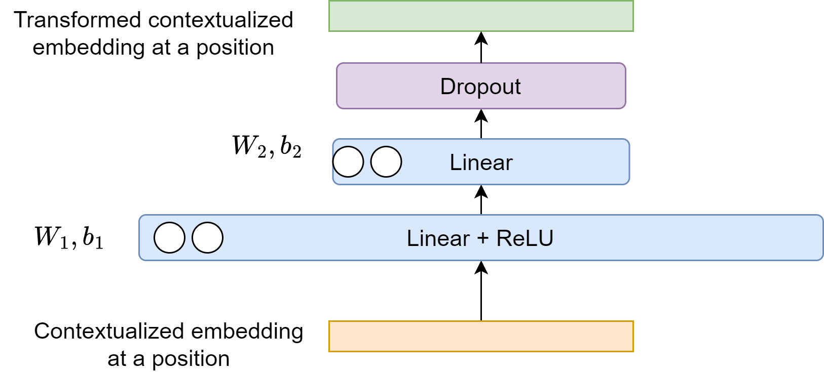
Fig. 5.4 Point-wise feed-forward network to perform nonlinear transformation on the contextualized embedding at each position. Residual connection and layer normalization are not shown.#
There are additional dropouts, residual connections, and layer normalization after the point-wise feed-forward layer. Taken all together, now we can define the following encoder layer.
Definition 5.1 (Encoder layer)
Given \(n\) sequential input embeddings represented as \(e_{in} = (e_{in,1},...,e_{in,n})\). The Transformer encoder layer performs the following calculation procedures
where \(e_{mid}, e_{out} \in \mathbb{R}^{n\times d_{model}}, \)
with \(W_1\in \mathbb{R}^{d_{model}\times d_{ff}}\), \(W_2\in \mathbb{R}^{d_{ff}\times d_{model}}\), \(b_1,b_2 \in \mathbb{R}^{d_{ff}}\), and the \(padMask\) excludes padding symbols in the sequence.
In a typical setting, we have \(d_{\text {model }}=512\), and the inner-layer has dimensionality \(d_{ff}=2048\).
Remark 5.2 (Is feedforward layer necessary for Transformer?)
Feedforward layer plays a critical role in introduce non-linearity and improving model capacity for Transformers.
While self-attention is powerful for capturing contextual relationships, it’s fundamentally a weighted linear sum operation.
If we stack multiple self-attention layers, the output vectors are still fundamentally a weighted linear sum of input vectors. With feedforward layer added after self-attention layer acting as non-linear transformation, the model capacity of transformer will increase as we stack more layers.
5.2.7. Encoder Computation Summary#
The whole computation in the encoder module can be summarized in the following.
Definition 5.2 (computation in encoder module)
Given an input sequence represented by integer sequence \(s = (i_1,...,i_p,...,i_n)\) and its position \(s^p = (1,..., p, ..., n)\). The encoder module takes \(s, s^p\) as inputs and produce \(e_N \in \mathbb{R}^{n\times d_{model}}\).
where \(e_i \in \mathbb{R}^{n\times d_{model}}\), \(\operatorname{EncoderLalyer}: \mathbb{R}^{n\times d_{model}}\to \mathbb{R}^{n\times d_{model}}\) is an encoder sub-unit, \(N\) is the number of encoder layers. Note that Dropout operations are not shown above. Dropouts are applied after initial embeddings \(e_0\), every self-attention output, and every point-wise feed-forward network output.
Also note that there is active research on where to optimally add the layer normalization in the encoder [XYH+20]. As shown in Fig. 5.5, post-layer normalization (the one in the original paper [VSP+17]) adds normalization layer after multi-head attention output and feed-forward layer output. Pre-layer normalization, on the other hand, adds normalization layer before the inputs entering into the multi-head attention and feed-forward layers.
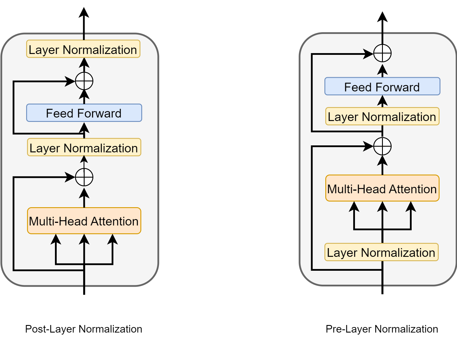
Fig. 5.5 Post-layer normalization and pre-layer normalization in an encoder layer.#
5.2.8. Decoder Anatomy#
In the decoder side, we are similarly given an output sequence represented by integer sequence \(o = (o_1,...,o_p,...,o_m), o_p\in \mathbb{N}\), \(e.g., o = (5, 10, 30, 2, ..., 21)\). The decoder module aims to converts an output sequence \(o\), combining with resulting embedding \(e_N\) in the encoder module to its corresponding probabilities over the vocabulary. The output probability can be used to compute categorical loss that drives the learning process of the encoder and the decoder.
Note that there are two type of attention in the decoder module, one is self-attention among the output sequence itself and one is attention between encoder output and decoder output, i.e., encoder-decoder attention. The encoder-decoder attention uses a mask that excludes padding symbol in the input sequence. The queries come from the output of previous sub-unit and keys and values come from the final output of the encoder module. This allows decoder sub-units to attend to all positions in the input sequence.
In each decoder layer, inputs are first contextualized via multi-head self-attention. Because we restrict each input token to only attend to its preceding input tokens, we apply a mask
The decoder self-attention uses a mask that excludes padding symbol and future symbol, which can be computed via logical \(\operatorname{OR}\) between \(padMask\) and \(seqMask\). \(seqMask\) for a symbol at position \(i\) is a binary vector \(seqMask_i \in \mathbb{R}^m\) whose value is 1 at position equal or greater than \(i\). Therefore, for a sequence of length \(m\), the complete \(seqMask\) would be a upper triangle matrix value 1.
Fig. 5.6 illustrates the connection between the Encoder component and Decoder component.
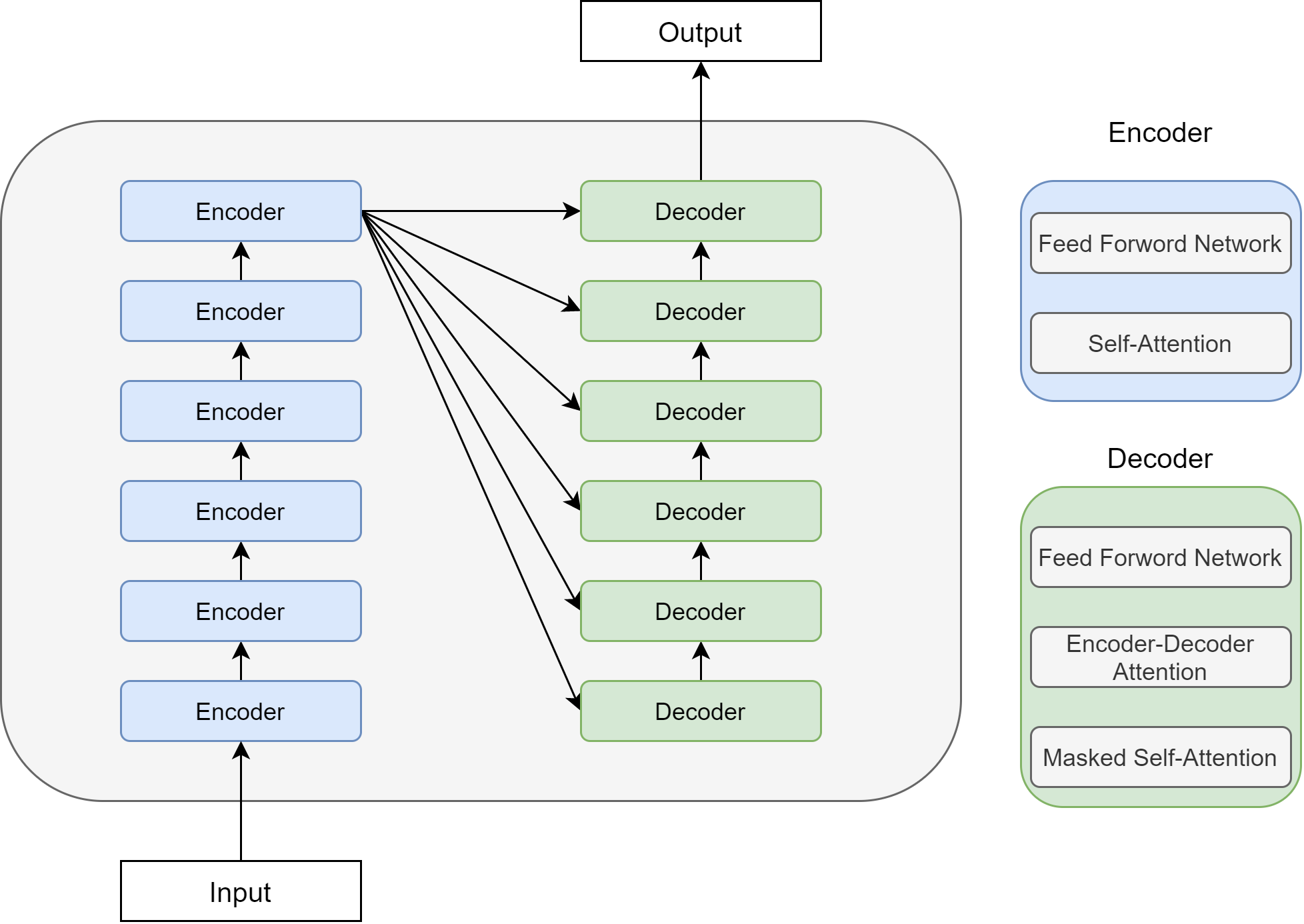
Fig. 5.6 Illustration of the interaction between encoder module output and deconder in Transformer.#
The whole computation in the decoder module can be summarized in the following.
Definition 5.3 (computation in decoder module)
Given an input sequence represented by integer sequence \(o = (o_1,...,o_p,...,o_n)\) and its position \(o^p = (1,..., p, ..., m)\). The encoder module takes \(o, o^p\) as inputs, combines final contextualized embedding \(e_N\) from the encoder, and produce \(d_N \in \mathbb{R}^{n\times d_{model}}\) and probabilities over the vocabulary.
where \(d_0 \in \mathbb{R}^{m\times d_{model}}\), \(\operatorname{DecoderLayer}: R^{m\times d_{model}}\to R^{m\times d_{model}}\) is a decoder sub-unit, \(N\) is the number of decoder sub-units, \(W\in\mathbb{R}^{ d_{model} \times |V|^O}\). Specifically, each decoder layer can be decomposed into following calculation procedures
where \(d_{mid1}, d_{mid2}, d_{out} \in \mathbb{R}^{m\times d_{model}}, \)
with \(W_1\in \mathbb{R}^{d_{model}\times d_{ff}}, W_2\in \mathbb{R}^{d_{ff}\times d_{model}}, b_1 \in \mathbb{R}^{d_{ff}}, b_2\in \mathbb{R}^{d_{model}}\).
5.2.9. Computational Breakdown Analysis#
In the following, we analyze the two core components of the Transformer (i.e., the self-attention module and the position-wise FFN). Let the model dimension be \(D\), and the input sequence length be \(T\). We also assume that the intermediate dimension of FFN is set to \(4D\) and the dimension of keys and values are set to \(D/H\) in the self-attention module.
The following data summarize the complexity and number of parameters for these two modules.
Module |
Complexity |
#Parameters |
|---|---|---|
self-attention |
\(O\left(T^2 \cdot D\right)\) |
\(4 D^2\) |
position-wise FFN |
\(O\left(T \cdot D^2\right)\) |
\(8 D^2\) |
Here are the key observations:
When the input sequences are short, the hidden dimension \(D\) dominates the complexity of self-attention and position-wise FFN. The bottleneck of Transformer thus lies in FFN.
When the input sequences grow longer, the sequence length \(T\) gradually dominates the complexity of these modules, in which case self-attention becomes the bottleneck of Transformer.
Furthermore, the computation of self-attention requires that a \(T \times T\) attention distribution matrix is stored, which makes the computation of Transformer to be memory bounded.
5.3. Different Branches Of Developments#
5.3.1. Overview#
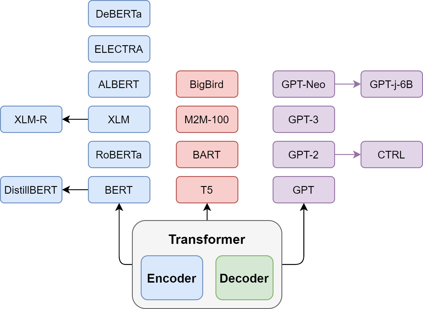
Fig. 5.7 Different branches of developments derived from the Transformer architecture: (left) Encoder branch, (middle) Encoder-Decoder branch, and (right) Decoder branch.#
The Transformer architecture was originally intended to tackle challenges in Seq2Seq tasks such as machine translation or summarization. The simplicity in architecture and effectiveness of attention mechanism draw much interest since its invention. Transformer type of architectures have become the dominant model architecture for most of NLP tasks. Moreover, Transformer architecture has also been widely adopted in computer vision [DBK+20] and recommender systems [SLW+19], which were previously by other CNN and DNN architectures.
In the process of adapting Transformer for different applications, there have been efforts that continue the improvement on the original encoder-decoder architecture as well as efforts that use only the encoder part or the decoder part separately.
For different branches of models, we employ different training strategies:
Generative pretrained models like the GPT family are trained using a Causal Language Modeling objective.
Denoising models like the BERT family are trained using a Masked Language Modeling objective.
Encoder-decoder models like the T5, BART or PEGASUS models are trained using heuristics to create pairs of (inputs, labels). These heuristics can be for instance a corpus of pairs of sentences in two languages for a machine translation model, a heuristic way to identify summaries in a large corpus for a summarization model or various ways to corrupt inputs with associated uncorrupted inputs as labels which is a more flexible way to perform denoising than the previous masked language modeling.
5.3.2. The Encoder Branch#
The most influential encoder-based model is BERT [DCLT18], which stands for Bidirectional Encoder Representations from Transformers. BERT is pretrained with the two objectives:
Predicting masked tokens in texts, known as masked language modeling (MLM)
Determining if two text passages follow each other, which is known as next-sentence-prediction (NSP).
The MLM helps learning of contextualized word-level representation, and the NSP objective aims to improve the tasks like question answering and natural language inference, which require reasoning over sentence pairs. BERT used the BookCorpus and English Wikipedia for pretraining and the model can then be fine-tuned with supervised data on downstream natural language understanding (NLU) tasks such as text classification, named entity recognition, and question-answering. At the time it was published, it achieved all state-of-the-art results on the popular GLUE benchmark. The success of BERT drew significant attention and up to date BERT like Encoder-only models dominate research and industry on natural language understanding (NLU) tasks [XWVD20]. We will discuss BERT in the following chapter.
RoBERTa (Robustly Optimized BERT) [LOG+19] is a follow-up study of BERT, which reveals that the performance of BERT can be further improved by modifying the pretraining scheme. RoBERTa uses larger batches with more training data and dropped the NSP task to significantly improve the performance over the original BERT model.
Although BERT model delivers great results, it can be expensive and difficult to deploy in production due to its model size and memory footprint. The ALBERT model [LCG+20] introduced three changes to make the encoder architecture more efficient. First, it reduces embedding dimensionality via matrix factorization, which saves parameters especially when the vocabulary gets large. Second, all layers share the parameters which decreases the number of effective parameters even further. Finally, ALBERT enhance the NSP objective with a more challenging sentence-ordering prediction (SOP), which primary focuses on inter-sentence coherence for sentence pairs in the same text segment.
By using model compression techniques like knowledge distillation, we can preserve most of the BERT performance with much smaller model size and memory footprint. Representative models include DistilBERT and TinyBERT.
5.3.3. The Decoder Branch#
The decoder component in the Transformer model can be used for auto-regressive language modeling. GPT series are among the most successful auto-regressive pretrained language models, and they form the foundation of LLM.
GPT-1 [RNSS18]: One of the major contributions of the GPT-1 study is the introduction of a two-stage unsupervised pretraining and supervised fine-tuning scheme. They demonstrates that a pre-trained model with fine-tuning can achieve satisfactory results over a range of diverse tasks, not just for a single task.
GPT-2 [RWC+19]: is a larger model trained on much more training data, called WebText, than the original one. It achieved state-of-the-art results on seven out of the eight tasks in a zero-shot setting in which there is no fine-tuning applied. The key contribution of GPT-2 is demonstrating the capability of zero-shot learning with extensively pretrained language model alone (i.e., no finetuning).
GPT-3 [BMR+20]: GPT-3 is up-scaled from GPT-2 by a factor of 100. It demonstrated that lead to significant improvements in performance and capabilities, which also marked the beginning of LLM era. Besides being able to generate impressively realistic text passages, the model also exhibits few-shot learning capabilities: with a few examples of a novel task such as text-to-code examples the model is able to accomplish the task on new examples.
5.3.4. The Encoder-decoder Branch#
Although it has become common to build models using a single encoder or decoder stack, there are several encoder-decoder variants of the Transformer that have novel applications across both NLU and NLG domains:
T5 The T5 model unifies all NLU and NLG tasks by converting all tasks into a text-to-text paradigm. As such all tasks are framed as sequence-to-sequence tasks where adopting an encoder-decoder architecture is natural. The T5 architecture uses the original Transformer architecture. Using the large crawled C4 dataset, the model is pre-trained with masked language modeling as well as the SuperGLUE tasks by translating all of them to text-to-text tasks. The largest model with 11 billion parameters yielded state-of-the-art results on several benchmarks although being comparably large.
BART BART combines the pretraining procedures of BERT and GPT within the encoder-decoder architecture. The input sequences undergoes one of several possible transformation from simple masking, sentence permutation, token deletion to document rotation. These inputs are passed through the encoder and the decoder has to reconstruct the original texts. This makes the model more flexible as it is possible to use it for NLU as well as NLG tasks and it achieves state-of-the-artperformance on both.
5.4. Bibliography#
Tom Brown, Benjamin Mann, Nick Ryder, Melanie Subbiah, Jared D Kaplan, Prafulla Dhariwal, Arvind Neelakantan, Pranav Shyam, Girish Sastry, Amanda Askell, and et al. Language models are few-shot learners. Advances in Neural Information Processing Systems, 33:1877–1901, 2020.
Jacob Devlin, Ming-Wei Chang, Kenton Lee, and Kristina Toutanova. Bert: pre-training of deep bidirectional transformers for language understanding. arXiv preprint arXiv:1810.04805, 2018.
Alexey Dosovitskiy, Lucas Beyer, Alexander Kolesnikov, Dirk Weissenborn, Xiaohua Zhai, Thomas Unterthiner, Mostafa Dehghani, Matthias Minderer, Georg Heigold, Sylvain Gelly, and others. An image is worth 16x16 words: transformers for image recognition at scale. arXiv preprint arXiv:2010.11929, 2020.
Zhenzhong Lan, Mingda Chen, Sebastian Goodman, Kevin Gimpel, Piyush Sharma, and Radu Soricut. Albert: a lite bert for self-supervised learning of language representations. 2020. URL: https://arxiv.org/abs/1909.11942, arXiv:1909.11942.
Jian Li, Zhaopeng Tu, Baosong Yang, Michael R Lyu, and Tong Zhang. Multi-head attention with disagreement regularization. arXiv preprint arXiv:1810.10183, 2018.
Yinhan Liu, Myle Ott, Naman Goyal, Jingfei Du, Mandar Joshi, Danqi Chen, Omer Levy, Mike Lewis, Luke Zettlemoyer, and Veselin Stoyanov. Roberta: a robustly optimized bert pretraining approach. arXiv preprint arXiv:1907.11692, 2019.
Alec Radford, Karthik Narasimhan, Tim Salimans, and Ilya Sutskever. Improving language understanding by generative pre-training. URL https://s3-us-west-2. amazonaws. com/openai-assets/researchcovers/languageunsupervised/language understanding paper. pdf, 2018.
Alec Radford, Jeffrey Wu, Rewon Child, David Luan, Dario Amodei, and Ilya Sutskever. Language models are unsupervised multitask learners. OpenAI Blog, 1(8):9, 2019.
Fei Sun, Jun Liu, Jian Wu, Changhua Pei, Xiao Lin, Wenwu Ou, and Peng Jiang. Bert4rec: sequential recommendation with bidirectional encoder representations from transformer. In Proceedings of the 28th ACM international conference on information and knowledge management, 1441–1450. 2019.
Ashish Vaswani, Noam Shazeer, Niki Parmar, Jakob Uszkoreit, Llion Jones, Aidan N Gomez, Łukasz Kaiser, and Illia Polosukhin. Attention is all you need. In Advances in neural information processing systems, 5998–6008. 2017.
Patrick Xia, Shijie Wu, and Benjamin Van Durme. Which* bert? a survey organizing contextualized encoders. arXiv preprint arXiv:2010.00854, 2020.
Ruibin Xiong, Yunchang Yang, Di He, Kai Zheng, Shuxin Zheng, Chen Xing, Huishuai Zhang, Yanyan Lan, Liwei Wang, and Tieyan Liu. On layer normalization in the transformer architecture. In International Conference on Machine Learning, 10524–10533. PMLR, 2020.