9. LLM Architecture Fundamentals

9.1. Overview

LLM have revolutionized natural language processing and artificial intelligence, demonstrating remarkable capabilities in understanding and generating human-like text. Tech companies like Google, Microsoft, Meta, OpenAI are producing LLMs with increasing sizes and capabilities just over the past few years [Fig. 9.1].

From a high level, LLMs share the following characteristics:

• Scale: LLMs are trained on enormous datasets, often containing hundreds to thousands of billions of words or tokens. This massive scale allows them to capture intricate patterns and nuances in language. For example, GPT-3 [BMR+20] was trained on about 500 billion tokens, and recent Llama3 405B [DAJ24] was trained on 15.6T tokens.

• Transformer architecture: Most modern LLMs use transformer architectures, which were introduced in the “Attention is All You Need” paper. These models can have billions of parameters - GPT-3 has 175 billion, for instance. The transformer architecture allows for efficient parallel processing and captures long-range dependencies in text.

• Self-supervised learning: LLMs are typically pre-trained using self-supervised learning techniques. The most common approach is next-token prediction, where the model learns to predict the next word in a sequence given the previous words. This allows the model to learn from vast amounts of unlabeled text data.

• Multi-task capability: A single LLM can perform various language tasks such as translation, summarization, question-answering, reasongin, and text generation without needing separate models for each task. This versatility makes them powerful tools for a wide range of applications.

• Few-shot learning via prompting: The multi-task ability of LLMs can often be simply invoked by prompting with a few examples provided in the prompt. This “in-context learning” allows them to adapt to new tasks without model weight update.

• Emergent reasoning abilities: As LLMs grow in size and complexity, they often develop capabilities that were hard to acquire among small models, for example, arithmetic reasoning and logical reasoning: Models may show ability to follow simple logical arguments or solve puzzles.

• Hallucination: LLMs can sometimes generate text that sounds plausible but is factually incorrect. This hallucination behavior is a significant challenge in deploying LLMs for applications requiring high reliability.

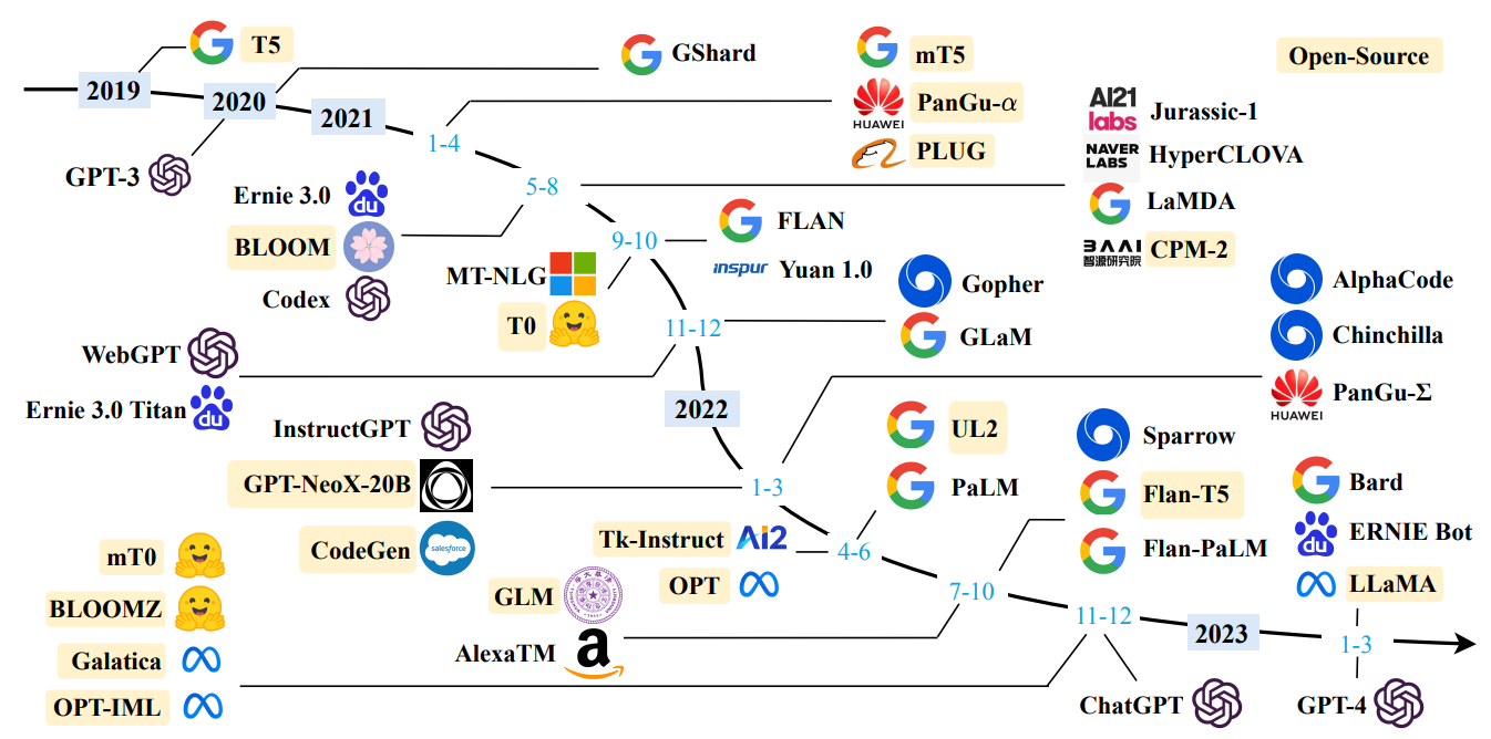
Fig. 9.1 A timeline of existing large language models (having a size larger than 10B) in recent years. We mark the open-source LLMs in yellow color. Image from [ZZL+23].

This chapter aims to go over the core components and architectural considerations that form the foundation of modern LLMs.

We begin by examining layer normalization, a crucial technique that stabilizes the learning process and allows for training of very deep networks, enhancing the overall performance of LLMs.

Next, we review the activation functions commonly used in LLM age, discussing their properties and impact on model performance and training dynamics.

The self-attention mechanism, a cornerstone of transformer models, is explored in depth, along with its variants that have emerged to address specific challenges or improve efficiency in processing and understanding context.

Next we cover position encoding techniques that allow transformer models to understand the sequential nature of language, with a focus on methods for handling long context – a critical challenge in scaling LLMs to process extensive inputs.

Finally, we examining the intricate details of LLM structure and function. We break down the distribution of parameters across different model components, provide a detailed explanation of the forward pass computation, and present examples of dense transformer architectures.

9.2. Layer Normalization

9.2.1. Layer normalization basics

The LayerNorm was originally proposed to overcome the internal covariate shift issue [IS15], where a layer’s input distribution changes as previous layers are updated, causing the difficulty of traning deep models.

The key idea in LayerNorm is to normalize the input distribution to the neural network layer via

• re-centering by subtracting the mean;

• re-scaling by dividing the standard deviation.

The calculation formula for an input vector \(x\) with \(H\) feature dimension is given by

(9.1)\[ \operatorname{LayerNorm}(x) =\frac{x-\mu}{\sqrt{\sigma+\epsilon}} \cdot \gamma+\beta \]

where

• \(\mu\) is the mean across feature dimensions, i.e., \(\mu = \frac{1}{H} \sum_{i=1}^H x_i \).

• \(\sigma\) is the standard deviation across feature dimensions, i.e., \(\sigma =\sqrt{\frac{1}{H} \sum_{i=1}^H\left(x_i-\mu\right)^2+\epsilon}\).

• \(\epsilon\) is a small number acting as regularizer for division.

• \(\gamma\) and \(\beta\) are learnable scaling and shifting parameters.

Remark 9.1 (Why we need \(\gamma\) and \(\beta\))

\(\gamma\) and \(\beta\) are parameters used to enhance the model’s learning capacity. As the normalization operation is used to stablize the learning by standardizing the data distribution, it also smooths out useful feature distributions and decreases the model’s learning capacity. With learnable shift and scaling parameters, we offset these negative impacts of normalization.

9.2.2. RMS Norm (Root Mean Square Norm)

RMSNorm [ZS19] is a technique aiming to achieve similar model training stablizing benefit with a reduced computational overhead compared to LayerNorm. RMSNorm hypothesizes that only the re-scaling component is necessary and proposes the following simplified normalization formula

(9.2)\[ \operatorname{RMSNorm}(x)=\frac{x}{\sqrt{\frac{1}{H} \sum_{i=1}^H x_i^2}} \cdot \gamma \]

where \(\gamma\) is learnable scaling parameter. Note that since we don’t normalize the mean, we don’t need need a learnable shift parameter like what is in the LayerNorm. Experiments show that RMSNorm can achieve on-par performance with LayerNorm with much reduced training cost.

In the following, we summarize the differences between RMSNorm and LayerNorm

Computational complexity

LayerNorm involves both mean and variance calculation for each normalization layer, which brings sizable computational cost for high-dimensional inputs in LLM (e.g., GPT-3 \(d_model = 12288\)). RMSNorm, on the other hand, only keeps the variance calculation, reducing the normalization cost by half.

Gradient propogation

LayerNorm stablizes the input distribution between layers through normalization and benefits deep networks training by alleviating the problem of vanishing or exploding gradients. However, LayerNorm can also be affected by noise and input shifts when calculating the mean, potentially leading to unstable gradient propagation. RMSNorm, by using only RMS for normalization, can provide a more robust, smoother gradient flow, especially in deeper networks. It reduces the impact of mean on gradient fluctuations, thereby improving the stability and speed of training.

See [ZS19] for math derivation

9.2.3. Layer normalization position

It has been shown in [XYH+20] that the position of normalization layer has an impact on model training, covergence, and final performance.

The Post-Norm (as in the vanilla Transformer architecture) can stablize the variance of the output by applying the LayerNorm after the residual connection, which is given by

\[\operatorname{PostNorm Output} = \operatorname{LayerNorm}(X + \operatorname{SubLayer}(X))\]

Here the SubLayer refers to either the FeedForward Layer or the Attention Layer.

The Pre-Norm normalizes the input to each SubLayers, which is given by

\[\operatorname{PreNorm Output} = X + \operatorname{SubLayer}(\operatorname{LayerNorm}(X)).\]

It is shown in [XYH+20] that the gradients at the last layer \(L\) satisfy the following condition:

\[||G_{PostNorm,L}||_F \leq \mathcal{O}(d \sqrt{\ln d}), ||G_{PreNorm,L}||_F \leq \mathcal{O}\left(d \sqrt{\frac{\ln d}{L}}\right) .\]

which intuitively implies the following

• The gradient norm magnitude in the Pre-Norm Transformer will be likely to stay the same for any layer index \(l\)

• Gradient norm in the Post-Norm Transformer will likely increase as layer index \(l\) and be very large at the last layer \(L\).

Such gradient norm behavior has implication on training stability.

• For Post-norm model, it often requires learning rate scheduling and warm up (initializing from a small vaue) to stablize training.

• When it comes to training very deep models, Post-norm can lead to more unstable gradients during training, especially in very deep networks. This can lead to slower convergence and increased likelihood of training failure.

• On the other hand, Pre-Norm Transformers without the warm-up stage can reach comparable results with Post-Norm, simplifying the hyper-parameter tuning;

• Pre-Norm, thanks to its stable gradient, is suitable for LLM architecture, which are usually very deep transformers.

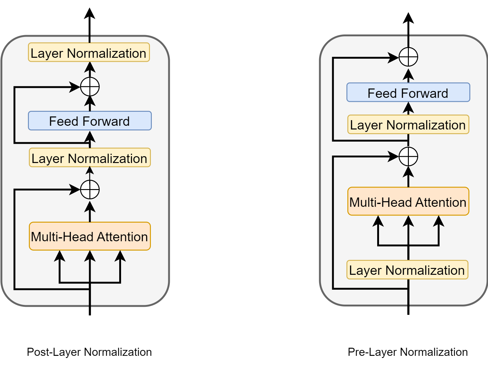
Fig. 9.2 Post-layer normalization and pre-layer normalization in an encoder layer.

Pre-Norm

• In the Pre-Norm architecture, the normalization operation (RMS Norm or Layer Norm) is performed before the self-attention or feed-forward neural network (FFN) calculations. In other words, the input to each layer is first normalized before being passed to the attention or feed-forward layers.

• Pre-Norm ensures that the magnitude of inputs remains within a stable range in deep networks, which is particularly beneficial for models with long-range dependencies. By performing normalization operations early, the model can learn from more stable inputs, thus helping to address the problem unstable gradients in deep models.

• LLMs like GPT, LLama are using Pre-Norm design

Post-Norm

• In the Post-Norm architecture, the normalization operation is performed after the self-attention or FFN calculations. The model first goes through unnormalized operations, and finally, the results are normalized to ensure balanced model outputs.

• Post-Norm can achieve good convergence effects in the early stages of training, performing particularly well in shallow models. However, in deep networks, the drawback of Post-Norm is that it may lead to gradient instability during the training process, especially as the network depth increases, gradients may become increasingly unstable during propagation.

Another modification of Post-Norm to enable training of very deep Post-Norm Transformer model (up to 1000 layers) is Deep-Norm [WMD+22], which gives

\[\operatorname{DeepNorm Output} = \operatorname{LayerNorm}(\alpha X + \operatorname{SubLayer}(X))\]

Here \(\alpha > 1\) is a constant, which up scales the residual connection (to help gradient vanishing issue for deep models). Besides, the weights in the SubLayers are scaled by \(\beta < 1\) (i.e., make it smaller) during initalization.

9.2.4. Layer normalization example choices

The core advantages of RMS Pre-Norm lie in its computational simplicity and gradient stability, making it an effective normalization choice for deep neural networks, especially large language models. This is exampified by the fact that recent LLaMa series started to use Pre-RMSNorm whereas GPT-3 model used Pre-LayerNorm.

• Improved computational efficiency: As RMS Norm omits mean calculation, it reduces the computational load for each layer, which is particularly important in deep networks. Compared to traditional Layer Norm, RMS Norm can process high-dimensional inputs more efficiently.

• Enhanced gradient stability: RMS Pre-Norm can reduce instances of vanishing gradients, especially in deep networks. This normalization method improves training efficiency by smoothing gradient flow.

• Suitable for large-scale models: For models like LLaMA, RMS Pre-Norm supports maintaining a relatively small model size while ensuring powerful performance. This allows the model to maintain good generalization capabilities without increasing complexity.

9.3. Nonlinearity in FFN

As introduced in Pointwise FeedForward Layer, the FFN block plays a critical role in improving model capacity via nonlinear activations.

Let \(x\) be the input vector, \(W_1, b_1\) and \(W_2, b_2\) be the weight matrices and biases for the two layers, the FFN block is given by

\[ \operatorname{FFN}(x)=f(xW_1+b_1)W_2+b_2, \]

where \(f\) is the activation function.

While ReLU is used in the vanilla Transformer model, many other different nonlinear activations are explored. In the latest LLMs, GLU activations [Sha20] are widely adopted and its variations SwiGLU are also widely used to achieve better performance in practice.

Gated Linear Units (GLU) is a neural network layer defined as the componentwise product of two linear transformations of the input, one of which is sigmoid-activated.

(9.3)\[\operatorname{GLU}(x; W, V, b)=\sigma(xW+b) \otimes xV \]

where \(W, V\) are weight matrices and \(b\) is the bias. Note that intuitively GLU introduces a gating mechanism on the product \(xV\) via the sigmoid function \(\sigma(xW+b)\). Such gating mechanism allows the model to learn when to emphasize or de-emphasize certain features.

Apply GLU in the FFN block, we yield

(9.4)\[ \operatorname{FFN}_{GLU}(x; W_1,W_2,V, b_1, b_2)=(\sigma(xW_1 + b) \otimes xV)W_2 + b_2 \]

where \(W_1, W_2, V\) are weight matrices. Note that the FFN layer with GLU have three weight matrices, as opposed to two for the original FFN.

One important variant of GLU is Swish [RZL17], which is given by

(9.5)\[ \operatorname{Swish}_\beta(x)=x \cdot \sigma(\beta x) \]

where \(\beta\) is a hyperparameter for Swish. Compared to GLU, Swish is a self-gated activation function. As showed in Fig. 9.3, Swish has the following appealing properites:

• Smooth derivative leading to better gradient flow, while ReLU is nonsmooth at \(x=0\)

• Non-monotonicity: The non-monotonic nature of Swish allows it to capture more complex relationships in the data

• Unbounded above and bounded below, whereas GLU is bounded above and below

• Non-zero gradient for negative inputs: For very negative inputs, Swish has a small but non-zero gradient, unlike ReLU which has a zero gradient. This can help mitigate the “dying ReLU” problem.

• Self-gating property allows the network to learn when to emphasize or de-emphasize certain features.

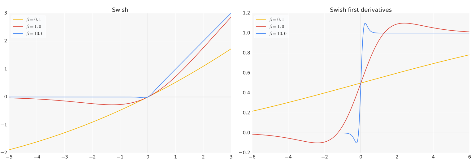
Fig. 9.3 (Left) The Swish activation function. (Right) First derivatives of Swish. Image from [RZL17].

If we use Swish function in the GLU, we can obtain the following SwiGLU and SwiGLU-FFN variations:

(9.6)\[\begin{split} SwiGLU=\text{Swish}_1(xW) \otimes xV \\ \operatorname{FFN}_{SwiGLU} = (\underbrace{\text{Swish}_1(xW_1)}_{\text{Gate Projection}}\otimes \underbrace{xV}_{\text{Up Projection}} ) \underbrace{W_2}_{\text{Down Projection}} \end{split}\]

with \(\operatorname{Swish}_1(x)=x \cdot \sigma(x)\).

Example activation in recent LLMs:

LLM	Activation Function
Mistral	SwiGLU
LLaMA	SwiGLU
Qwen	SwiGLU

9.4. Self-attention Variants

9.4.1. Multi-Head Attention (MHA)

Multi-Head Attention [detailed in Multihead Attention with Masks] is the foundation of many Transformer-based models, including the original Transformer architecture.

The computation of an \(H\)-headed MHA given input \(X\in \mathbb{R}^{n\times d_{model}}\) matrix and \(H\) projection matrices \(W^Q_i, W^K_i, W^V_i \in\mathbb{R}^{d_{model}\times d_{head}}\), \(i\in \{1,...,H\}\) is given by

\[ \text{MultiHead}(Q, K, V) = \text{Concat}(\text{head}_1, ..., \text{head}_H)W^O \]

where each head is computed as:

\[ \text{head}_i = \text{Attention}(XW^Q_i, XW^K_i, XW^V_i) \]

with the attention given by

\[ \text{Attention}(Q, K, V) = \text{Softmax}(\frac{QK^T}{\sqrt{d_{head}}})V. \]

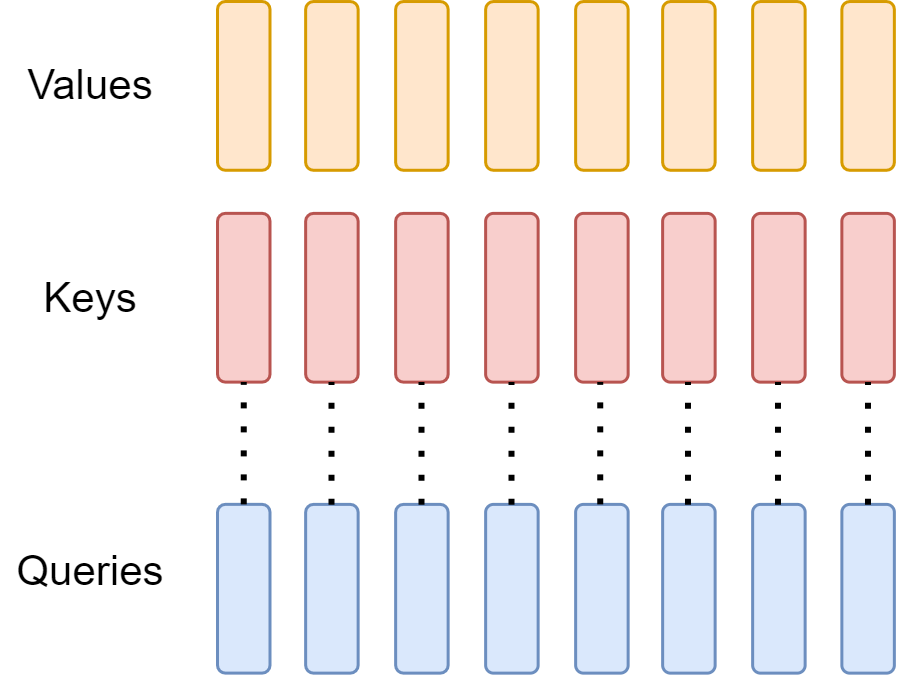
Fig. 9.4 Multi-head attention has \(H\) query, key, and value heads for each token.

Remark 9.2 (Combine to RoPE)

More recent LLMs are using Rotary Position Embedding (RoPE) (see Rotary Postion Embedding). The position information related to the query key \(Q_i\) (row \(i\) from \(Q\))at position \(i\) and the key \(K_j\) at position \(j\) is baked in through

\[\tilde{Q}_i = Q_i\mathcal{R}_i, \tilde{K}_j = K_j\mathcal{R}_j.\]

Here \(\mathcal{R}_i\) is a rotation matrix parameterized by position integer \(i\).

Finally, the Attention computation is computed using the rotated query and key, given by

\[ \text{Attention}(Q, K, V) = \text{Softmax}(\frac{\tilde{Q}\tilde{K}^T}{\sqrt{d_{head}}})V. .\]

In the following, we summarize the advantages and drawbacks of MHA.

Advantages

• Improves the model’s overall learning capacity

• Different heads allow the model to jointly attend to information from different representation subspaces

Drawbacks

• Computational complexity scales quadratically with sequence length (i.e., huge cost for long context applications)

• During inference stage, each head has its own key and value to cache (i.e., KV cache), bring additional memory burden to inference process.

9.4.2. Multi Query Attention (MQA)

To reduce the inference cost from MHA, [Sha19] proposed MQA, which reduces \(H\) key and value heads in MHA to a single key and value shared head. During inference, MQA reduces the size of the key-value cache by a factor of \(H\) (see KV Cache). However, larger models generally scale up the number of heads (e.g., GPT-2 has 12 heads; GPT-3 has 96 heads), such that MQA represents a very aggressive cut in both memory bandwidth and capacity footprint.

In MQA, the single head attention is computed as

\[ \text{head}_i = \text{Attention}(XW^Q_i, XW^K, XW^V). \]

Note that we only have one group of \(W^K, W^V\) matrices.

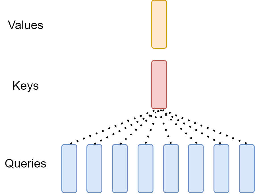
Fig. 9.5 Multi-head attention has \(H\) query, and one shared single key head and single value head for each token.

MQA often comes at the cost of quality degradation. In the following, we summarize the MHA advantages and drawbacks.

Advantages

• During inference stage, each head has its own key and value to cache, bring additional memory burden to inference process.

Drawbacks

• Computational complexity scales quadratically with sequence length (i.e., huge cost for long context applications)

• Modeling capacity is largely compromised due to the reduction of multiple heads to single head, leading to quality degradation.

9.4.3. Grouped Query Attention (GQA)

GQA [ALTdJ+23] is an optimization of MHA and MQA that aims to reduce computational complexity while maintaining performance.

Unlike MQA, GQA uses an intermediate (more than one, less than number of query heads) number of key-value heads. GQA is shown to achieve quality close to MHA, but with comparable inference speed to MQA.

In GQA, the single head attention is computed as

\[ \text{head}_i = \text{Attention}(QW^Q_i, KW^K_{g(i)}, VW^V_{g(i)}) \]

Here \(g(i)\) is a function that maps head index to group index (e.g., \(g(1): \{1, 2\} \to \{1\}\)) and we have \(G\) groups of \(W^K,W^V\) matrices.

Studies [Fig. 9.6] show that GQA (with \(G <= 8\)) can improve latency by reducing parameters and computation compared to MHA and at the same time maintain most of the performance of MHA.

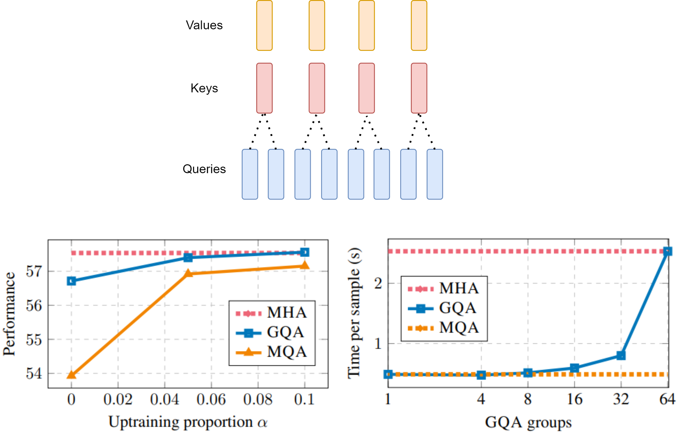
Fig. 9.6 (Top) GQA divides the key and value heads into multiple groups. Within each group, a single shared key and value heads are attended to by query heads. GQA interpolats between MHA and MQA. (Bottom) GQA-8 performance and latency compared with MHA and MQA. Image from [ALTdJ+23]

GQA is widely adopted in the latest LLM. Following shows example configurations of Qwen2 and Mistral LLM series [JSM+23, YYHBZ24].

Table 9.1 Model configuration of Qwen2 and Mistral, which uses GQA (# KV heads is number of groups )

Configuration	Hidden Size	# Layers	# Query Heads	# KV Heads
Qwen2 0.5B	896	24	14	2
Qwen2 1.5B	1,536	28	12	2
Qwen2 7B	3,584	28	28	4
Qwen2 72B	8,192	80	64	8
Mistral 7B	4096	32	32	8

9.4.4. Multi-Head Latent Attention (MLA)

9.4.5. Sliding Window Attention

The computational complexity for MHA, MQA, GQA are scaling quadratically with the sequence length. This constrains the context length that LLM can effectively process, impacting their ability to handle long documents or maintain coherence over extended generations.

To address this challenge, recent LLMs (e.g., Mistral [JSM+23]) adopts sliding window attention, which reduces the computational complexity by restricting each token’s attention to a fixed-size window \(W\) of preceding tokens, rather than attending to the entire sequence. The computational complexity is reduced from quadratic \(O(s^2)\) to linear \(O(\min(W, s)\times s)\), where \(s\) is the sequence length. Although the token can only capture local context within its fixed window, with multiple layers stacked upon each other, a token at layer \(L\) can effectively attend to previous \(L\times W\) tokens.

In Mistral 7B with \(L = 32\), and \(W\) set to 4096, the effective attention length is about \(131K\) tokens.

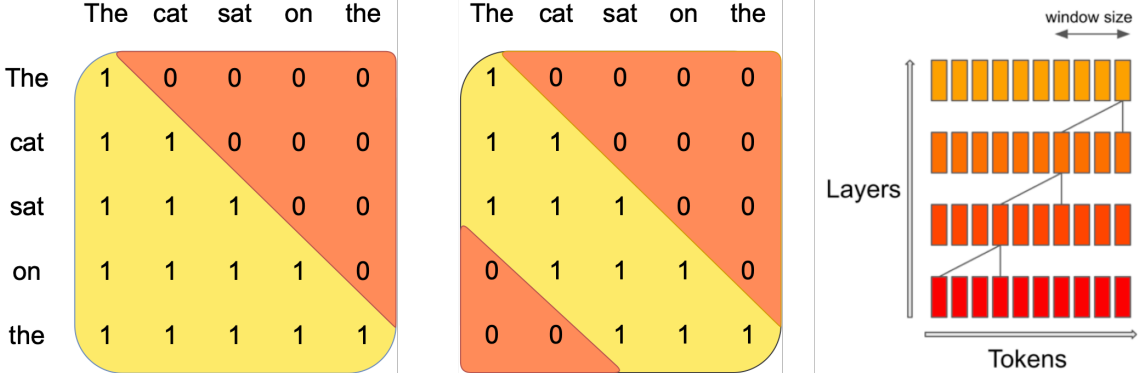
Fig. 9.7 Illustration of sliding window attention (Middle), which restrict each token to attend at most \(W\) preceding tokens. As a comparison, MHA (Left) attends to all the preceding tokens. While at each layer the information flow is limited by window size, after \(L\) layers, information can flow forward by up to \(L\times W\) tokens. Image from [JSM+23]

9.5. Position Encoding and Long Context

9.5.1. Motivation

Context window in LLM represents the number of input tokens the model can process simultaneously when responding in the prompt. GPT-4 has a context window of approximately \(32k\) or roughly 25,000 words. Recent advancements have extended this to more than 100k (e.g., Llama3) or even 1 million (Gemini), which is about 8 average length English novels.

A longer context window allows the model to process and understand more information before generating a response, providing a deeper grasp of the context. This capability is especially useful when inputting a large amount of specific data into a language model and asking questions about it. For instance, when analyzing an extensive document about a particular company or issue, a larger context window enables the language model to review and retain more of this detailed information, leading to more accurate and customized responses.

9.5.2. Absolute Position Encoding

In Position Encodings, we discuss absolute position encoding, which maps an integer \(i\) (used to represent the position of the token) to a \(d_{model}\) sinusoidal vector. Specifically, let \(PE(i)_j\) represent the \(j\)th dimention position encoding, we have

\[\begin{split} \operatorname{PE}(i)_j = \left\{\begin{array}{l} \sin \left(w_j i\right), \quad \text { if } j \text{ is even} \\ \cos \left(w_j i\right), \quad \text { if } j \text{ is odd} \end{array}\right. \end{split}\]

where \(w_j=1/10000^{j / d_{model}}\) if \(j\) is even and \(w_j=1/10000^{j-1 / d_{model}}\) if \(j\) is odd and \(j=0,...,d_{model} - 1\).

While absolute position encoding has achieved success in BERT, it has several key issues when it is applied in LLMs:

• Lack of extrapolation due to limited sequence length: Models are restricted to a maximum sequence length during training (e.g., BERT 512), limiting their ability to generalize to positions beyond the maximum length at inference time.

• Position insensitivity: The position encoding is added on top of token embedding and go through linear projection before interacting with other tokens, instead of directly interacting with other tokens during attention score computation.

• Lack of invariance to shift: For two tokens with fixed relative position disance, their interaction at attention score computation layer is dependent on their absolute position. For relative position encodings, this property is by construction.

9.5.3. ALiBi

ALiBi (Attention with Linear Biases) [PSL22] is a simple approach that suprisinly addresses all drawbacks in the sinusoidal abolute position encoding above. The key idea is to simply add a static, relative position dependent bias into the Softmax computation step [Fig. 9.8]. Specifically, for the attention weight between query token \(i\) to all the key vectors, we have

\[\operatorname{AttentionWeight} = \operatorname{Softmax}(\underbrace{Q_iK^T/d_{Head}}_{\text{scaled query-key doc product}} + \underbrace{m \cdot[−(i − 1), ..., −2, −1, 0]}_{\text{ALiBi bias vector}}) \]

where scalar \(m\) is a head-specific slope hyperparameter fixed before training (e.g., for a model with 8 heads, \(1/2, 1/2^2,...,1/2^8\)).

Note that AliBi has the following nice property by construction:

• It is a relative position encoding

• Long distance decay, tokens with larger distance have smaller impact.

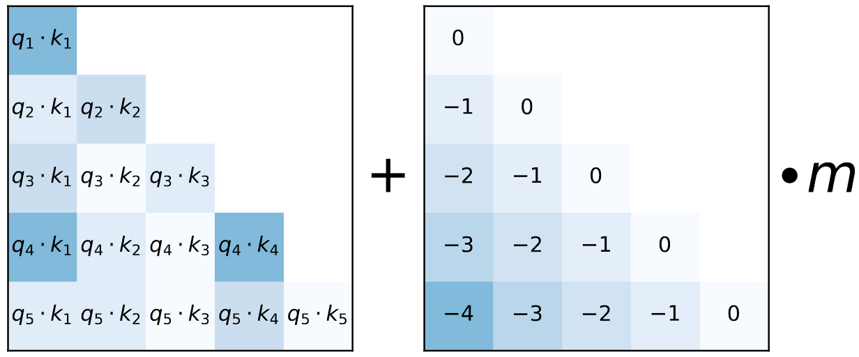
Fig. 9.8 When computing attention weights for each head, ALiBi adds a constant bias (Right) to each attention score ($Q_iK^T), with scaling factor omitted (Left). Image from [PSL22].

Compare with sinusoidal absolute position encoding baseline [Fig. 9.9], there are several advantages of Alibi:

• When train and validate on the same input token length \(L\), Alibi shows advantages over baseline.

• When train on shorter length (e.g., 512), but validate on longer (e.g., 1024,…,3072), Alibi method extropolates well.

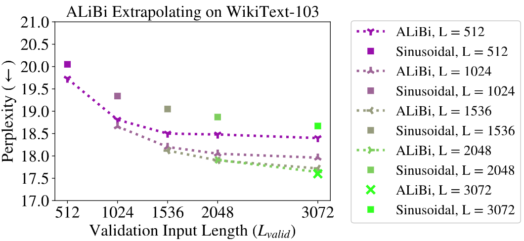
Fig. 9.9 Comparision between the ALiBi models trained and evaluated on varying sequence lengths on the WikiText-103 validation set and the sinusoidal absolute position encoding baseline. Image from [PSL22].

9.5.4. Rotary Postion Embedding

9.5.4.1. The mechanism

Rotary Position Encoding (RoPE) [SLP+23] is a widely adopted and proved-effective position encoding method in latest LLM (e.g., Llama, Qwen, etc.). RoPE has ideas similar to ALiBi and sinusoid position encoding:

• Like ALiBi, relative positional information is directly used in attention score computation.

• Sinusoid functions are used in construction for their nice mathematical properties.

Specifically, the key idea of RoPE is to multiply query vector \(Q_m\) (of a token at position \(m\)) and key vector \(K_n\) (of another token at position \(n\)) by a rotational matrix \(\mathcal{R}(m; \Theta)\) and \(\mathcal{R}(n; \Theta)\) before taking the scaled doc product. Here rotational matrix \(\mathcal{R}(\cdot; \Theta)\) is constructed a group of 2D rotational matrices, whose wave-length are specified by \(\Theta\).

The \(d_{model}\times d_{model}\) rotational matrix for position \(m\) is given by

\[\begin{split} \mathcal{R}_{\Theta, m}=\left(\begin{array}{ccccccc} \cos m \theta_1 & -\sin m \theta_1 & 0 & 0 & \cdots & 0 & 0 \\ \sin m \theta_1 & \cos m \theta_1 & 0 & 0 & \cdots & 0 & 0 \\ 0 & 0 & \cos m \theta_2 & -\sin m \theta_2 & \cdots & 0 & 0 \\ 0 & 0 & \sin m \theta_2 & \cos m \theta_2 & \cdots & 0 & 0 \\ \vdots & \vdots & \vdots & \vdots & \ddots & \vdots & \vdots \\ 0 & 0 & 0 & 0 & \cdots & \cos m \theta_{d / 2} & -\sin m \theta_{d / 2} \\ 0 & 0 & 0 & 0 & \cdots & \sin m \theta_{d / 2} & \cos m \theta_{d / 2} \end{array}\right) \end{split}\]

Here the rotary matrix has pre-defined parameters \(\Theta=\left\{\theta_i=10000^{-2(i-1) / d}, i \in[1,2, \ldots, d_{model} / 2]\right\}\), which can be interpreted as wave length from \(2\pi\) (when \(i = 1\)) to \(10000 \cdot 2\pi\) (when \(i = d_{model}/2\)). Intuitively,

• Short wave length is used to capture the high-frequency, short-ranged information in positions.

• Long wave length is used to capture low-frequency, long-range information in position.

Pre-SoftMax input (omitting scaling) for query token at position \(m\) and key token at position \(n\) is given by

\[ \operatorname{PreSoftmax}(Q_m, K_n) =\left( Q_m \mathcal{R}_{\Theta, m}\right) \cdot \left( K_n \mathcal{R}_{\Theta, n} \right) \]

Example 9.1

For \(d_{model} == 2\), the rotation matrix for position \(m \) is:

\[\begin{split} \mathcal{R}(m; \Theta)=\left[\begin{array}{cc} \cos (m\theta_1) & -\sin (m\theta_1) \\ \sin (m\theta_1) & \cos (m\theta_1) \end{array}\right] \end{split}\]

Where \(\theta_1 = 1\).

For \(d_{model} == 4\), the rotation matrix for position \(m \) is:

\[\begin{split} \mathcal{R}(m; \Theta)=\left[\begin{array}{cc} \cos (m\theta_1) & -\sin (m\theta_1) & 0 & 0 \\ \sin (m\theta_1) & \cos (m\theta_1) & 0 & 0 \\ 0 & 0 & \cos (m\theta_2) & -\sin (m\theta_2) \\ 0 & 0 & \sin (m\theta_2) & \cos (m\theta_2) \end{array}\right] \end{split}\]

Where \(\theta_1 = 1, \theta_2 = 10000^{-2/4}\).

9.5.4.2. Properties of RoPE

Relative position encoding: Now we are showing that the rotated query-key inner product is a function of the relative position in 2D cases (the conclusion can be generalized to high-dimensional rotational matrix). Specifically, let \(\theta_q = m\theta\) and \(\theta_k = n\theta\), where \(m\) and \(n\) are integer positions of query vector token and key vector token.

\[\begin{split} \begin{aligned} \left\langle \mathcal{R}\left(\theta_q\right) Q_m, \mathcal{R}\left(\theta_k\right) K_n\right\rangle & =Q_m^{\top} \mathcal{R}\left(\theta_q\right)^{\top} \mathcal{R}\left(\theta_k\right) K_n \\ & =Q_m^{\top} \mathcal{R}\left(\theta_k-\theta_q\right) K_n \\ & =\left\langle \mathcal{R}\left(\theta_q-\theta_k\right) Q_m, K_n\right\rangle \\ & =\left\langle \mathcal{R}\left(\theta (m-n)\right) Q_m, K_n\right\rangle \end{aligned} \end{split}\]

That is, the Pre-Softmax input of \(Q_m, K_n\) is a funciton of \(m - n\).

We have used the following important properties of rotational matrix:

1. The transpose of a rotation matrix is equal to its inverse: \(\mathcal{R}(\theta)^{\top}=\mathcal{R}(-\theta)\).

2. The matrix multiplication of rotational matrices satisfies: \(\mathcal{R}(\theta_x)\cdot \mathcal{R}(\theta_y) = \mathcal{R}(\theta_x + \theta_y)\)

In other words, the inner product of two rotated vectors is equal to the inner product of one vector rotated by their angle difference and the other original vector.

Long-term decay: In [SLP+23], it is shown that the inner-product will decay when the relative position increase. This property aligns with desired property that a pair of tokens will have gradually descreasing semantic impact on each other when they are far apart.

9.5.5. Extending Context Windows via RoPE

9.5.5.1. Position Interpolation for RoPE

Position Interpolation[CWCT23] is a cheap method to extend the context window of an existing LLM, which allows LLM to have longer context window during inference time than the context window size used during training.

The idea is to linearly down-scales the input position indices to match the original context window size [Fig. 9.10].Specifically, given that the rotation matrix in RoPE is a continuous function, one can adjust the rotation matrix for large position \(m\) to \(m'\) as

\[\mathcal{R}_{\Theta, m} = \mathcal{R}_{\Theta, m'}, m' = \frac{L}{L'}\]

where \(L\) maximum length of context window during the training and \(L' > L\) is larger context window we would like to apply during the inference stage. Intuitively, we reduce position indices from \(\left[0, L^{\prime}\right)\) to \([0, L)\) to match the original range of indices before computing RoPE.

It is found that Position Interpolation is highly effective and efficient, requiring only a very short period of fine-tuning for the model to fully adapt to greatly extended context windows. For example, extending the initial context window of 2048 to 32768 only requires fine-tuning for 1000 steps on the Pile.

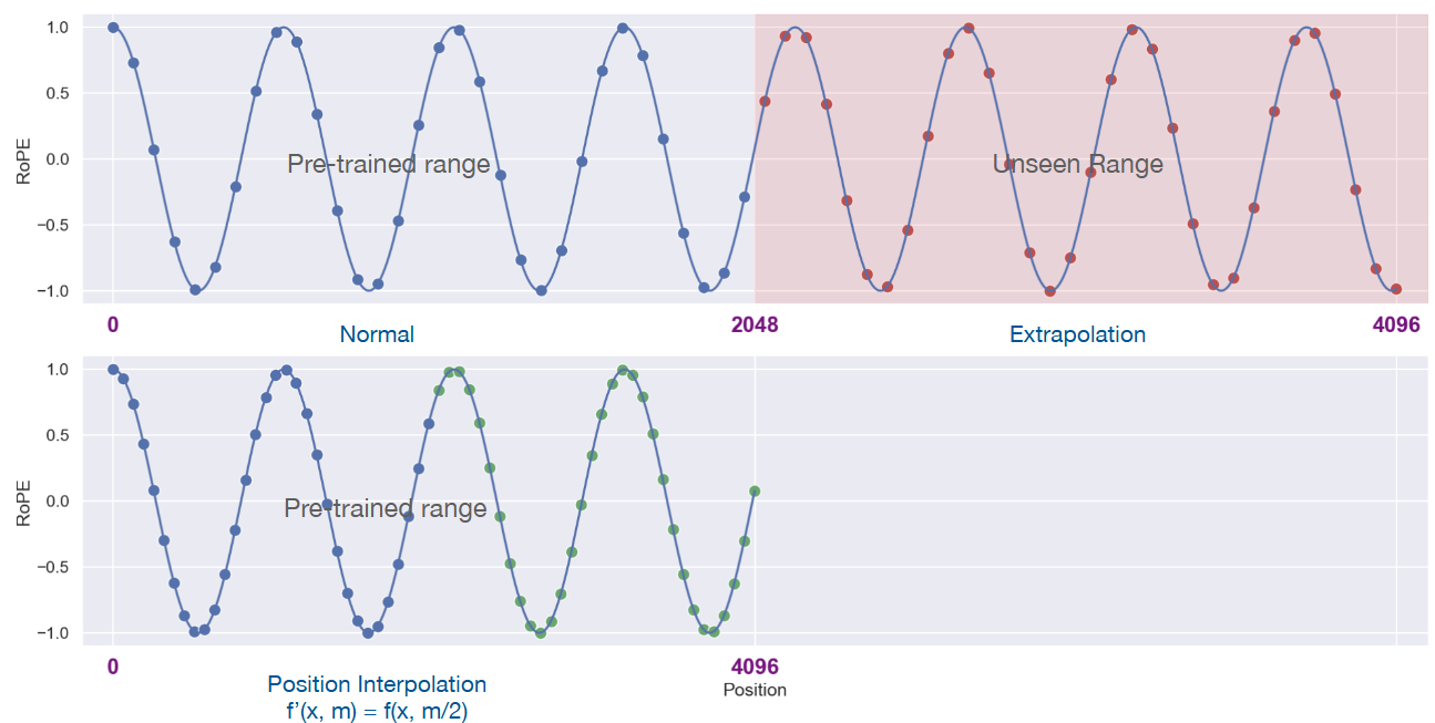
Fig. 9.10 An illustration of the Position Interpolation method, which is used to extend an initial context window from 2048 to 4096. Image from [CWCT23].

9.5.5.2. NTK-Aware RoPE

From the information encoding (i.e., Neural Tangent Kernel - NTK theory) perspective, the scaling by Position Interpolation uniformly scales wave length by a factor of \(L'/L\), which can hurt the model’s ability in capture high-frequency, short-ranged position information after rescaling.

The NTK-aware interpolation was proposed in public as a reddit post. Instead of scaling the wave length of every dimension uniformly, we scale up short wavelength less and long wavelength more.

More precisely, let the scaling factor be \(s=L^{\prime} / L\) and \(b\) be the original base. We perform a base change as follows:

\[ b^{\prime}=b \cdot s^{\frac{|d_{model}|}{|d_{model}|-2}} . \]

Note that the wave length at dimention \(i\) is given \(\lambda = 2\pi b^{2i/d_{model}}\). To see the scaling-up effect is larger on dimensions with large wavelength (i.e., large \(i\)), we have

\[\begin{split} \begin{align*} \log \frac{\lambda'}{\lambda} &= 2 i d_{model} (\log b' - \log b) \\ &= 2 i d_{model} (\frac{|d_{model}|}{|d_{model}|-2} \log s) \end{align*} \end{split}\]

which is a monontically increasing function on \(i\) given that \(d_{model}\) and \(s\) are constants.

9.5.5.3. NTK-by-parts and YaRN

9.5.5.4. Dual Chunk Attention

Dual Chunk Attention [AHZ+24] applies the chunking idea to map the position distance \((i - j)\) between a query state at position \(i\) and and a key state at position \(j\) to a value within the training stage context window size \(L\).

More specifically, let the \(M(i, j)\) be the mapping function of dual chunk attention. \(M\) has hyperparameter of chunk size \(s < L\) and local context window size \(w = L - s\), which is given by

\[\begin{split} M(i, j)= \begin{cases}P_{\mathbf{q}}^{\text {Intra }}[i]-P_{\mathbf{k}}[j] & \text { if }\lfloor i / s\rfloor-\lfloor j / s\rfloor=0 \\ P_{\mathbf{q}}^{\text {Succ }}[i]-P_{\mathbf{k}}[j] & \text { if }\lfloor i / s\rfloor-\lfloor j / s\rfloor=1 \\ P_{\mathbf{q}}^{\text {Inter }}[i]-P_{\mathbf{k}}[j] & \text { if }\lfloor i / s\rfloor-\lfloor j / s\rfloor>1 .\end{cases} \end{split}\]

Here

• \(P_{\mathbf{q}}^{\text {Intra }}[i] = P_{\mathbf{k}}[i] = i \bmod s\)

• \(P_{\mathbf{q}}^{\text {Inter }}[i] = L - 1 \)

• \(P_{\mathbf{q}}^{\text {Succ }} = (s, s+1,...,s + w - 1, L-1,...,L-1) \)

Intutiviely,

• When \(i\) and \(j\) are within the same chunk, i.e., \(|i - j| <= s\), \(M(i, j) = i - j\), which recovers the original position distance.

• When \(i\) and \(j\) have a distance of at least two chunks, \(i\) is capped at the value of \(L - 1\) and \(j = j \bmod s\).

• When \(i\) and \(j\) are within two consecutive chunks separately, a smoothed mapping is used to preverse locality.

To summarize, DCA consists of three components: (1) intra-chunk attention, which recover the same attention when two positions are within the same chunk; (2) inter-chunk attention for tokens between distinct chunks; and (3) successive chunk attention for processing tokens residing in two consecutive distinct chunks.

9.6. Tokenziation, vocabulary, and weight tying

9.6.1. BPE Tokenization

Byte Pair Encoding (BPE) is a commonly used subword tokenization algorithm in NLP [SHB15]. It starts with individual characters and iteratively merges the most frequent pairs to create new subword units, repeating this process N times to build the final subword vocabulary. The following is a summary of the algorithm.

Algorithm 9.1 (BPE)

Inputs Word list \(W\), Number of desired merges \(N\)

Output Subword vocabulary \(V = \emptyset\)

1. Represent each word as a sequence of characters

2. Initialize the subword vocabulary as a set of single characters

3. For i in 1 to N: 3.1 Calculate the frequency of each consecutive character pair 3.2 Find the character pair \((x, y)\) with the highest frequency 3.3 Merge the character pair \(c = (x, y)\), update the subword vocabulary \(V = V \cup c\).

4. Return the subword vocabulary \(V\).

Example 9.2

GPT-2’s vocabulary size is 50,257, corresponding to 256 basic byte tokens, a special end-of-text token, and 50,000 tokens obtained through merging process.

9.6.2. From BPE to BBPE

BPE (Byte Pair Encoding) and BBPE (Byte-level BPE) are both subword tokenization following the same idea of merging algorithm Algorithm 9.1 but operating on different granularities.

In short, BPE works on character or unicode level whereas BBPE works on byte level of UTF-8 representation. Their comparison is summarized as the following.

BPE

In BPE, the generation of subwords is more consistent with linguistic rules (e.g., utilizing word roots). The subword choices often better align with common vocabulary.

However, it often requires different treatments for different languages (like English vs Chinese) and it cannot effectively represent emojis and unseen special tokens.

BBPE

BBPE has following advantages:

• It can process all character sets (including Unicode characters), making it suitable for multilingual scenarios.

• It provides good support for unconventional symbols and emojis.

However, as BBPE is working on smaller granularity level than characters, it might result in larger vocabulary size (i.e., larger embedding layers) and unnatural subword units.

Currently, many mainstream large language models (such as the GPT series, Mistral[1], etc.) primarily use BBPE instead of BPE. The reasons for the widespread adoption of this method include:

• Ability to process multilingual text: Large models typically need to handle vast amounts of text in different languages. BBPE operates at the byte level, allowing it to process all Unicode characters, performing particularly well for languages with complex character sets (such as Chinese, Korean, Arabic).

• Unified tokenization: The BBPE method does not rely on language-specific character structures. Therefore, it can be uniformly applied to multilingual tasks without adding extra complexity, simplifying the tokenization process in both pre-training and downstream tasks.

• Compatibility with emojis and special characters: Modern large language models need to process large amounts of internet data, which contains many emojis, special characters, and non-standard symbols. BBPE can better support these types of symbols.

Remark 9.3 (What does Byte-level mean?)

“Byte-level” in the context of BBPE means that the algorithm operates on individual bytes of data rather than on characters or higher-level text units. Note that characters are typically encoded using schemes like UTF-8, where a single character might be represented by one or more bytes. In other words, BBPE treats the input as a sequence of raw bytes, without interpreting them as characters or considering character boundaries.

Below is more context about UTF-8 encoding.

1. ASCII encoding:

   • In the original ASCII encoding, each character is represented by a single byte (8 bits).

   • This allows for 256 different characters (2^8 = 256).

   • ASCII mainly covers English letters, numbers, and some basic symbols.

2. Unicode and UTF-8:

   • Unicode was developed to represent characters from all writing systems in the world.

   • UTF-8 is a variable-width encoding scheme for Unicode.

   • In UTF-8, characters can be encoded using 1 to 4 bytes:

     • ASCII characters still use 1 byte

     • Many other characters use 2 or 3 bytes

     • Some very rare characters use 4 bytes

3. Examples:

   • The letter ‘A’ (U+0041 in Unicode) is represented as a single byte: 01000001

   • The Euro symbol ‘€’ (U+20AC) is represented by three bytes: 11100010 10000010 10101100

   • The emoji ‘😊’ (U+1F60A) is represented by four bytes: 11110000 10011111 10011000 10001010

This multi-byte representation for single characters is why text processing algorithms that work at the character level can be more complex than those that work at the byte level, especially when dealing with multilingual text.

9.7. Parameter composition in Transformer models

In this section, we do an accounting exercise by estimating the number of parameters in a Transformer model. This will give us some insight on

• which component makes up the majority of parameters and

• how the total number of parameters scales when we scale up different components.

Let \(V\) be the vocabulary size, \(d\) be the model hidden dimensions, \(L\) be the number of layer,

Table 9.2 Parameters in a Transformer

Module	Computation	Parameter Name	Shape	Parameter Number
Attention	\({Q} / {K} / {V}\) projection	weight / bias	\([{d}, {d}] /[{d}]\)	\(3 d^2+3 d\)
	Attention output projection	weight / bias	\([{d}, {d}] /[{d}]\)	\(d^2+d\)
	Layernorm	\(\gamma, \beta\)	\([{d}] /[{d}]\)	\(2 d\)
FFN	First layer up-projection	weight / bias	\([{d}, 4 {~d}] /[{d}]\)	\(4 d^2+d\)
	Second layer down-projection	weight / bias	\([4 {~d}, {~d}] /[4 {~d}]\)	\(4 d^2+4 d\)
	Layernorm	\(\gamma, \beta\)	\([{d}] /[{d}]\)	\(2 d\)
Embedding (tied)	-	-	\([{V}, {d}]\)	\(V d\)
Total				\(V d+L\left(12 d^2+13 d\right)\)

The key scaling properties from this table are:

• The total number of parameters scales linearly with number of layers \(L\)

• The total number of parameters scales quadratically with model hidden dimensionality \(d\).

Remark 9.4

We have simplification in the above computation for MHA but the results are the same. Suppose we have \(H\) heads, head dimension \(d_{head}\) and \(H \times d_{head} = d\). QKV transformation matrices have weight parameters \(3 \times H \times d \times d_{head} = 3d^2\).

With GQA that has \(G\) key-value shared heads, the total parameters are \(d^2 + 2Gd_{head}d\).

Example 9.3

Take the following GPT-3 13B and 175B as an example, 175B model has approximate 2.4 times of \(L\) and \(d_{model}\). Extrapolating from 13B model, we estimate the 175B model to have model parameters of \(13\times 2.4^3 = 179B\), which is very close.

Model Name	\(n_{\text{params}}\)	\(L\)	\(d\)	\(H\)	\(d_{head}\)
GPT-3 13B	13.0B	40	5140	40	128
GPT-3 175B or “GPT-3”	175.0B	96	12288	96	128

9.8. Forward Pass Computation Breadown

In this section, we estimate the computational cost (in term of FLOPS) for a forward pass.

Remark 9.5 (FLOPs estimation)

If \(A \in R^{m \times k}, B \in R^{k \times n}\) then, to compute \(A B\) the number of floating-point arithmetic required is \(2 m n k\).

For example, for

\[\begin{split}A = \begin{bmatrix}a_{11} & a_{12} \\ a_{21} & a_{22}\end{bmatrix}, B = \begin{bmatrix}b_{11} & b_{12} \\ b_{21} & b_{22}\end{bmatrix},\end{split}\]

The resulting \(C = AB\) has \(k\) terms, which are given by

\[c_{ij} = \sum_{t=1}^k a_{ik}b_{kj}.\]

It is clear that for each \(c_{ij}\) there are \(k\) multiplications and \(k\) additions (technically \(k-1\) additions among \(k\) terms).

Let \(V\) be the vocabulary size, \(b\) be the batch size, \(s\) be sequence length, \(d\) be the model hidden dimensions, \(L\) be the number of layer, we have summarized the computation breakdown in the following.

Table 9.3 Computation breakdown

Module	Computation	Matrix Shape Changes	FLOPs
Attention	\({Q} / {K} / {V}\) Projection	\([{b}, {s}, {d}] \times [{~d}, {~d}]\to[{b}, {s}, {d}]\)	\(3\times 2 b s d^2\)
	\(Q K^T\) dot product	\([{~b}, {~s}, {~d}] \times [{~b}, {~d}, {~s}]\to[{b}, {s}, {s}]\)	\(2 b s^2 d\)
	Score Matrix \( \dot V\)	\([{~b}, {~s}, {~s}] \times [{~b}, {~s}, {~d}]\to[{b}, {s}, {d}]\)	\(2 b s^2 d\)
	Output (with \(W_o\))	\([{b}, {s}, {d}] \times[{~d}, {~d}]\to[{b}, {s}, {d}]\)	\(2 b s d^2\)
FFN	First layer up-projection	\([{~b}, {~s}, {~d}] \times[{~d}, 4 {~d}] \to [{b}, {s}, 4 {~d}]\)	\(8 b s d^2\)
	Second layer down-projection	\([{~b}, {~s}, 4 {~d}] \times[4 {~d}, {~d}]\to[{b}, {s}, {d}]\)	\(8 b s d^2\)
Embedding		\([{b}, {s}, 1] \times[{~V}, {~d}]\to[{b}, {s}, {d}]\)	\(2 b s d V\)
In total			\(\left(24 b s d^2+4 b d s^2\right) \times L+2 b s d V\)

The key scaling properties from this table are:

• The total compute scales linearly with number of layers \(L\), and number of batch size \(b\)

• The total compute scales quadratically with model hidden dimensionality \(d\) and input sequence length \(s\).

9.9. Dense Architecture Examples

9.10. Bibliography

Good reviews [ZZL+24]

[ALTdJ+23] (1,2)

Joshua Ainslie, James Lee-Thorp, Michiel de Jong, Yury Zemlyanskiy, Federico Lebrón, and Sumit Sanghai. Gqa: training generalized multi-query transformer models from multi-head checkpoints. 2023. URL: https://arxiv.org/abs/2305.13245, arXiv:2305.13245.

[AHZ+24]

Chenxin An, Fei Huang, Jun Zhang, Shansan Gong, Xipeng Qiu, Chang Zhou, and Lingpeng Kong. Training-free long-context scaling of large language models. arXiv preprint arXiv:2402.17463, 2024.

[BMR+20]

Tom Brown, Benjamin Mann, Nick Ryder, Melanie Subbiah, Jared D Kaplan, Prafulla Dhariwal, Arvind Neelakantan, Pranav Shyam, Girish Sastry, Amanda Askell, and et al. Language models are few-shot learners. Advances in Neural Information Processing Systems, 33:1877–1901, 2020.

[CWCT23] (1,2)

Shouyuan Chen, Sherman Wong, Liangjian Chen, and Yuandong Tian. Extending context window of large language models via positional interpolation. arXiv preprint arXiv:2306.15595, 2023.

[DAJ24]

Abhimanyu Dubey and et al Abhinav Jauhri. The llama 3 herd of models. 2024. URL: https://arxiv.org/abs/2407.21783, arXiv:2407.21783.

[IS15]

Sergey Ioffe and Christian Szegedy. Batch normalization: accelerating deep network training by reducing internal covariate shift. 2015. URL: https://arxiv.org/abs/1502.03167, arXiv:1502.03167.

[JSM+23] (1,2,3)

Albert Q. Jiang, Alexandre Sablayrolles, Arthur Mensch, Chris Bamford, Devendra Singh Chaplot, Diego de las Casas, Florian Bressand, Gianna Lengyel, Guillaume Lample, Lucile Saulnier, Lélio Renard Lavaud, Marie-Anne Lachaux, Pierre Stock, Teven Le Scao, Thibaut Lavril, Thomas Wang, Timothée Lacroix, and William El Sayed. Mistral 7b. 2023. URL: https://arxiv.org/abs/2310.06825, arXiv:2310.06825.

[PSL22] (1,2,3)

Ofir Press, Noah A. Smith, and Mike Lewis. Train short, test long: attention with linear biases enables input length extrapolation. 2022. URL: https://arxiv.org/abs/2108.12409, arXiv:2108.12409.

[RZL17] (1,2)

Prajit Ramachandran, Barret Zoph, and Quoc V. Le. Searching for activation functions. 2017. URL: https://arxiv.org/abs/1710.05941, arXiv:1710.05941.

[SHB15]

Rico Sennrich, Barry Haddow, and Alexandra Birch. Neural machine translation of rare words with subword units. arXiv preprint arXiv:1508.07909, 2015.

[Sha19]

Noam Shazeer. Fast transformer decoding: one write-head is all you need. 2019. URL: https://arxiv.org/abs/1911.02150, arXiv:1911.02150.

[Sha20]

Noam Shazeer. Glu variants improve transformer. 2020. URL: https://arxiv.org/abs/2002.05202, arXiv:2002.05202.

[SLP+23] (1,2)

Jianlin Su, Yu Lu, Shengfeng Pan, Ahmed Murtadha, Bo Wen, and Yunfeng Liu. Roformer: enhanced transformer with rotary position embedding. 2023. URL: https://arxiv.org/abs/2104.09864, arXiv:2104.09864.

[WMD+22]

Hongyu Wang, Shuming Ma, Li Dong, Shaohan Huang, Dongdong Zhang, and Furu Wei. Deepnet: scaling transformers to 1,000 layers. 2022. URL: https://arxiv.org/abs/2203.00555, arXiv:2203.00555.

[XYH+20] (1,2)

Ruibin Xiong, Yunchang Yang, Di He, Kai Zheng, Shuxin Zheng, Chen Xing, Huishuai Zhang, Yanyan Lan, Liwei Wang, and Tieyan Liu. On layer normalization in the transformer architecture. In International Conference on Machine Learning, 10524–10533. PMLR, 2020.

[YYHBZ24]

An Yang, Baosong Yang, Binyuan Hui, and et al. Bo Zheng. Qwen2 technical report. 2024. URL: https://arxiv.org/abs/2407.10671, arXiv:2407.10671.

[ZS19] (1,2)

Biao Zhang and Rico Sennrich. Root mean square layer normalization. 2019. URL: https://arxiv.org/abs/1910.07467, arXiv:1910.07467.

[ZZL+23]

Wayne Xin Zhao, Kun Zhou, Junyi Li, Tianyi Tang, Xiaolei Wang, Yupeng Hou, Yingqian Min, Beichen Zhang, Junjie Zhang, Zican Dong, Yifan Du, Chen Yang, Yushuo Chen, Zhipeng Chen, Jinhao Jiang, Ruiyang Ren, Yifan Li, Xinyu Tang, Zikang Liu, Peiyu Liu, Jian-Yun Nie, and Ji-Rong Wen. A survey of large language models. arXiv preprint arXiv:2303.18223, 2023.

[ZZL+24]

Wayne Xin Zhao, Kun Zhou, Junyi Li, Tianyi Tang, Xiaolei Wang, Yupeng Hou, Yingqian Min, Beichen Zhang, Junjie Zhang, Zican Dong, Yifan Du, Chen Yang, Yushuo Chen, Zhipeng Chen, Jinhao Jiang, Ruiyang Ren, Yifan Li, Xinyu Tang, Zikang Liu, Peiyu Liu, Jian-Yun Nie, and Ji-Rong Wen. A survey of large language models. 2024. URL: https://arxiv.org/abs/2303.18223, arXiv:2303.18223.

---

[1]

See https://docs.mistral.ai/guides/tokenization/ for details for tokenizer construction and usage in Mistral LLMs.