19. Decoding

19.1. Decoding Fundamentals

In typical language modeling frameworks, a language model takes preceding words as context and outputs a probabilistic distribution of the next word over a pre-defined vocabulary. The overall goal of decoding is to convert the probabilistic outputs iteratively to generate a sequence of words that meet the requirement of intended applications.

Decoding introduces a few challenges that are vastly different from typical NLU (natural language understanding) tasks:

• The decoding involves iterative forword pass of a model taking updated inputs. As a result, decoding has significantly more computation cost than typical NLU tasks that simply involves one forward pass of a model.

• The quality (i.e., fluency and cohesion) and diversity of the generated text depends on the choice of language model, decoding methods, and their associated hyper-parameters.

At the heart of decoding is to maximize the probability of the generated sequence of tokens \(y_1,...,y_t\) given the input \(x\).

\[\hat{y} = \underset{y}{\operatorname{argmax}} P(y_1,...,y_t|x).\]

Since it is difficult optimize \(P(\mathbf{y} \mid \mathbf{x})\) directly, it is common to use the chain rule of probability to factorize it as a product of conditional probabilities

\[ P\left(y_1, \ldots, y_t \mid \mathbf{x}\right)=\prod_{t=1}^N P\left(y_t \mid y_{<t}, \mathbf{x}\right) \]

where \(y_{<t}\) is a shorthand notation for the sequence \(y_1, \ldots, y_{t-1}\). The problem of generating the most probable sequence now amounts to carefully selecting each word at each step given the preceding words in a sentence such that the probability of final sequence is maximized.

The model takes the sequence \(y_{<t}, \mathbf{x}\) as the input, and is trained to output the conditional probabilties of \(P\left(y_t \mid y_{<t}, \mathbf{x}\right)\).

19.1.1. Greedy decoding

The simplest decoding method is greedy decoding, in which we at each step greedily select the token with the highest model predicted probability:

\[ \hat{y}_t=\underset{y_t}{\operatorname{argmax}} P\left(y_t \mid y_{<t}, \mathbf{x}\right). \]

For example, suppose the language model produces a conditional probability \(p_{t, i}\) for token \(i\) in the vocabulary at step \(t\) given its preceding words, we will just take the token \(j\) that has the maximum value \(p_{t,j}\).

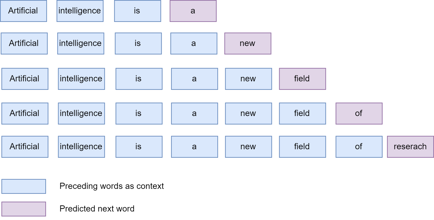
Fig. 19.1 Greedy decoding demonstrations.

While being efficient, greedy search decoding often fails to produce sequences that have high probability. The reason is that the token at each step is chosen without considering its impact on the subsequent tokens. In practice, the model may produce repetitive output sequences. This happens when the model identifies that certain words following each other with high probability. The root cause could be similar patterns are seen frequently during the pretraining stage.

In the following, we will introduce beam search and sampling methods to mitigate the drawbacks of greedy decoding.

19.1.2. Beam search decoding

19.1.2.1. Basics

Instead of decoding the token with the highest probability at each step, beam search keeps track of the top \(B\) most probable candidate sequences or hypotheses when selecting next-tokens. Here \(B\) is referred to the beam width or the number of hypotheses. By selecting the \(B\) next tokens from the vocabulary for extensions, we form \(B\) most likely new sequences as the next set of beams. This process is repeated until each sequence reaches the maximum length or an EOS token.

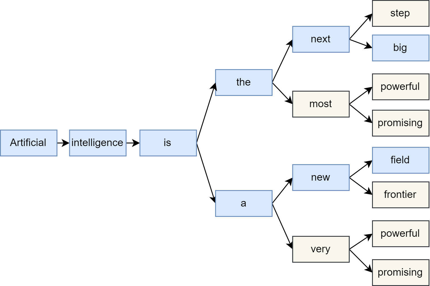
Fig. 19.2 Beam Search decoding demonstrations.

Formally, we denote the set of \(B\) hypotheses tracked by beam search at the start of step \(n\) as \(Y_{n-1}=\left\{\mathbf{y}_{1:n-1}^{(1)}, \ldots, \mathbf{y}_{1:n-1}^{(B)}\right\}\), where \(\mathbf{y}_{1:n-1}^{(j)}\) is hypothesis \(j\) consisting of \(n-1\) tokens. At each step, all possible single token extensions of these \(B\) beams given by the set \(\mathcal{Y}_n=Y_{n-1} \times \mathcal{V}\) and selects the \(B\) most likely extensions. At each step, we are selecting top \(B\) scored candidates from all \(B \times|\mathcal{V}|\) members of \(\mathcal{Y}_t\), given by

\[ Y_{n}=\underset{Y_{n} \in \mathcal{Y}_t}{\operatorname{argmax}} \operatorname{Score}\left(\mathbf{y}_{1:n}\right).\]

The most commonly used score function is the sum of negative log-likelihoods of the sequence, discounted by a length-related factor. For example,

\[ \operatorname{Score}\left(\mathbf{y}_{1:L}\right) = -\frac{1}{L^\alpha} \log P\left(y_1, \ldots, y_n \right)=-\frac{1}{L^\alpha} \sum_{n=1}^L \log P\left(y_{n} \mid y_1, \ldots, y_{n-1}\right) \]

where \(L\) is the length of candidate sequence and \(\alpha\) is a scalar (e.g., 0.75)tuning the length discount factor. Since a longer sequence has more terms in the summation and thus tend to get higher scores, the term \(L^\alpha\) in the denominator penalizes long sequences.

19.1.2.2. Computational complexity

Beam search has a computational complexity given by \(O(LB|V|)\), where

• \(L\) is the length of the sequence

• \(B\) is the beam width

• \(|V|\) is the vocabulary size (i.e., the search space size on each step).

In principle, beam search cannot guarantee the finding of optimal sequence, but it is much more effective than brute force apporach (which has time complexity of \(O(|V|^L)\)).

We can tune the diversity or length of generated text by incorporating other elements into the scoring function. For example, we can penalize long sequence by multiplying by log-likelihoods by a length-dependent factor.

19.1.2.3. Controling beam search behavior

Since beam-decoding is optimizing a user-defined score function, we can incorpoate various penalties or rewards into the score function to control the diversity, brevity, smoothness, etc. of the generated sequence[VCS+16]. For example,

• Let \(s\) be the original score, we can add length penalty by using score \(s\exp(-\alpha l)\), where \(\alpha\) is a scalar and \(l\) is the length of the generated sequence. \(\alpha > 0.0\) means that the beam score is penalized by the sequence length; \(\alpha < 0.0\) is used to encourage the model to generate longer sequence.

• We can use min_length to force the model to not produce an EOS (end of sentence) token before min_length is reached.

• One can also introduce n-grams repetition penalty. For example, one can specify a hard penalty to ensure that no n-gram appears twice. Alternatively, one can also introduce soft penalty\cite{keskar2019ctrl}. For instance, given a list of generated tokens \(G\), the probability distribution for the next token \(p_i\) is defined as:

\[ p_i=\frac{\exp \left(z_i /(T \cdot I(i \in g))\right.}{\sum_j \exp \left(z_j /(T \cdot I(j \in g))\right.} \]

where \(I(c)=\theta\) if \(c\) is True else 1.0.

Beam search aims to generate the most probable sequence, which however is not necessary of high quality from human language perspective. Human language does not necessarily follow a distribution of high probability next words, in particularly in creative writing or dialog generation. In other words, as humans, we want generated text to surprise us and not to be boring/predictable.

For applications like machine translation or summarization, we can specify beam search parameters to generate text of desired length. However, for tasks like story generation, the detailed length is often difficult to predict, which imposes a challenge to beam search.

19.2. Temperature-controlled sampling

19.2.1. The basics

Alternatively, we can look into stochastic approaches to avoid the response being generic. Instead of taking the tokens that deterministic maximizes the probability from the Softmax function, we can perform randomly sample the next token from the vocabulary according to probability of each token from the Softmax function. The temperature-controlled sampling randomly samples from the model output’s probability distribution over the full vocabulary at each step:

\[P(y_t=w_i | y_{<t}) = exp(z_{t,i} / T) / sum_{j=1}^{|V|} exp(z_{t,j} / T)\]

where \(z_{t_i}\) is the logit for token \(i\) at step \(t\), \(|V|\) denotes the cardinality of the vocabulary. We can easily control the diversity of the output by adding a temperature parameter T that rescales the logits before taking the Softmax. There are two special cases:

• When \(T \to 0\), the temperature-controlled sampling approaches a greedy decoding.

• When \(T \to \inf\), the temperature-controlled sampling approaches the uniformly sampling.

Setting the right temperature is critically to produce rich yet meaningful sentences. For example, a very high temperature would produce has produced mostly gibberish, including the appearance of many rare or even made-up words and uncommon grammar patterns.

19.2.2. Top-k and top-p sampling

Top-k and top-p sampling are two common extensions to the temperature-controlled sampling. The basic idea of both approaches is to impose additional constraints on the number of possible tokens we can sample from at each step.

The idea behind top-\(k\) sampling is used to ensure that the less probable words will not be considered at all and only top \(k\) probable tokens will be sampled. This imposes a fixed cut on the long tail of the word distribution and prevent the generation of rare words and going off-topic. One disadvantage of top-\(k\) sampling is that the number \(K\) need to be defined in the beginning. Selecting an universal \(K\) is non-trivial, as shown in the two following cases:

• When the next word has a broad distribution, having a small \(K\) will discard many reasonable options.

• When the next word has a narrow distribution, having a large \(K\) will cause the generation of rare words.

The top-\(p\) approach aims to adapt \(k\) heuristically based on the distribution shape. Let token \(i=1,...,|V|\) be sorted descendingly according to its probability \(p_i\). The top-p sampling approach chooses a probability threshold \(p_0\) and sets k to be the lowest value such that \(\sum_i (p_i) > p_0\). If the next word distribution is narrow (i.e., the model is confident in its next-word prediction), then k will be lower and vice versa.

19.3. Multi-step Decoding

19.3.1. Speculative Decoding

[CBI+23, LKM23, MOZ+23]

19.3.2. Multihead Decoding (Medusa)

[CLG+24]

19.4. Bibliography

[CLG+24]

Tianle Cai, Yuhong Li, Zhengyang Geng, Hongwu Peng, Jason D Lee, Deming Chen, and Tri Dao. Medusa: simple llm inference acceleration framework with multiple decoding heads. arXiv preprint arXiv:2401.10774, 2024.

[CBI+23]

Charlie Chen, Sebastian Borgeaud, Geoffrey Irving, Jean-Baptiste Lespiau, Laurent Sifre, and John Jumper. Accelerating large language model decoding with speculative sampling. arXiv preprint arXiv:2302.01318, 2023.

[LKM23]

Yaniv Leviathan, Matan Kalman, and Yossi Matias. Fast inference from transformers via speculative decoding. In International Conference on Machine Learning, 19274–19286. PMLR, 2023.

[MOZ+23]

Xupeng Miao, Gabriele Oliaro, Zhihao Zhang, Xinhao Cheng, Zeyu Wang, Zhengxin Zhang, Rae Ying Yee Wong, Alan Zhu, Lijie Yang, Xiaoxiang Shi, and others. Specinfer: accelerating generative large language model serving with tree-based speculative inference and verification. arXiv preprint arXiv:2305.09781, 2023.

[VCS+16]

Ashwin K Vijayakumar, Michael Cogswell, Ramprasath R Selvaraju, Qing Sun, Stefan Lee, David Crandall, and Dhruv Batra. Diverse beam search: decoding diverse solutions from neural sequence models. arXiv preprint arXiv:1610.02424, 2016.