4. Word Embeddings

4.1. Overview

Human language is structured through a complex combinations of different levels of linguistic building blocks such as characters, words, sentences, etc. Among different levels of these building blocks, words and its subunits (i.e., morphemes) are the most basic ones. Note: A morpheme is the smallest unit of language that has a meaning. Not all morphemes are words, but all prefixes and suffixes are morphemes. For example, in the word multimedia, multi- is not a word but a prefix that changes the meaning when put together with media. Multi- is a morpheme.

Many machine learning and deep learning approaches in natural language processing (NLP) requires explicit or implicit construction of word-level or subword level representationss. These word-level representations are used to construct representations of larger linguistic units (e.g., sentences, context, and knowledge), which are used to solve NLP tasks, ranging from simple ones such as sentiment analysis and search completion to complex ones such as text summerization, writing, question-answering, etc. Modern NLP tasks heavily hinge on the quality of word embedding and pre-trained language models that produce context-dependent or task dependent word representations.

NLP tasks are faced with text data consisting of tokens from a large vocabulary (\(>10^5-10^6\)). In sentiment analysis, we need to represent text data by numeric values such that computers can understand. One naive way to represent the feature of a word is the one-hot word vector, whose length of the typical size of the vocabulary.

Example 4.1

Consider a vocabulary of size \(V\), the one hot encodings for selected of words are represented as follows.

\[\begin{split} \begin{align*} \text { Rome } &= \underbrace{[1,0,0,0,0, 0, \ldots, 0]}_{length ~V}\\ \text { Paris } & =[0,1,0,0,0,0, \ldots, 0] \\ \text { America } & =[0,0,1,0,0,0, \ldots, 0] \\ \text { Canada } & =[0,0,0,1,0,0, \ldots, 0] \end{align*} \end{split}\]

One-hot sparse representation treats each word as an independent atomic unit that has equal distance to all other words. Such encoding does not capture the relations among words (i.e., meanings, lexical semantic) and lose its meaning inside a sentence. For example, consider three words run, horse, and cloth. Although run and horse tend to be more relevant to each other than horse and ship, they have same Euclidean distance. Additional disadvantage include its poor scalability, that is, its representation size grows with the size of vocabulary. As such one hot encodings are thus not considered as good features for advanced natural language processing tasks that draw on interactions and semantics among words, such as language modeling, machine learning. But there are exceptions when the vocabulary associated with a task is indeed quite small and words in the vocabulary are largely irrelevant to each other.

A much better alternative is to represent each word vector by a dense vector, whose dimensionality \(D\) typically ranges from 25 to 1,000.

Example 4.2

**Dense vector **representation for some words could be

\[\begin{split} \begin{align} \text { Rome } &= \underbrace{[0.1,0.3,-0.2,\ldots, 0]}_{length ~D}\\ \text { Paris } & =[-0.6,0.5,0.2, \ldots, 0.3] \\ \text { America } & =[0.3,0.2,-0.3, \ldots, 0.2] \\ \text { Canada } & =[0.15,0.2,0.4, \ldots, 0.1]. \end{align} \end{split}\]

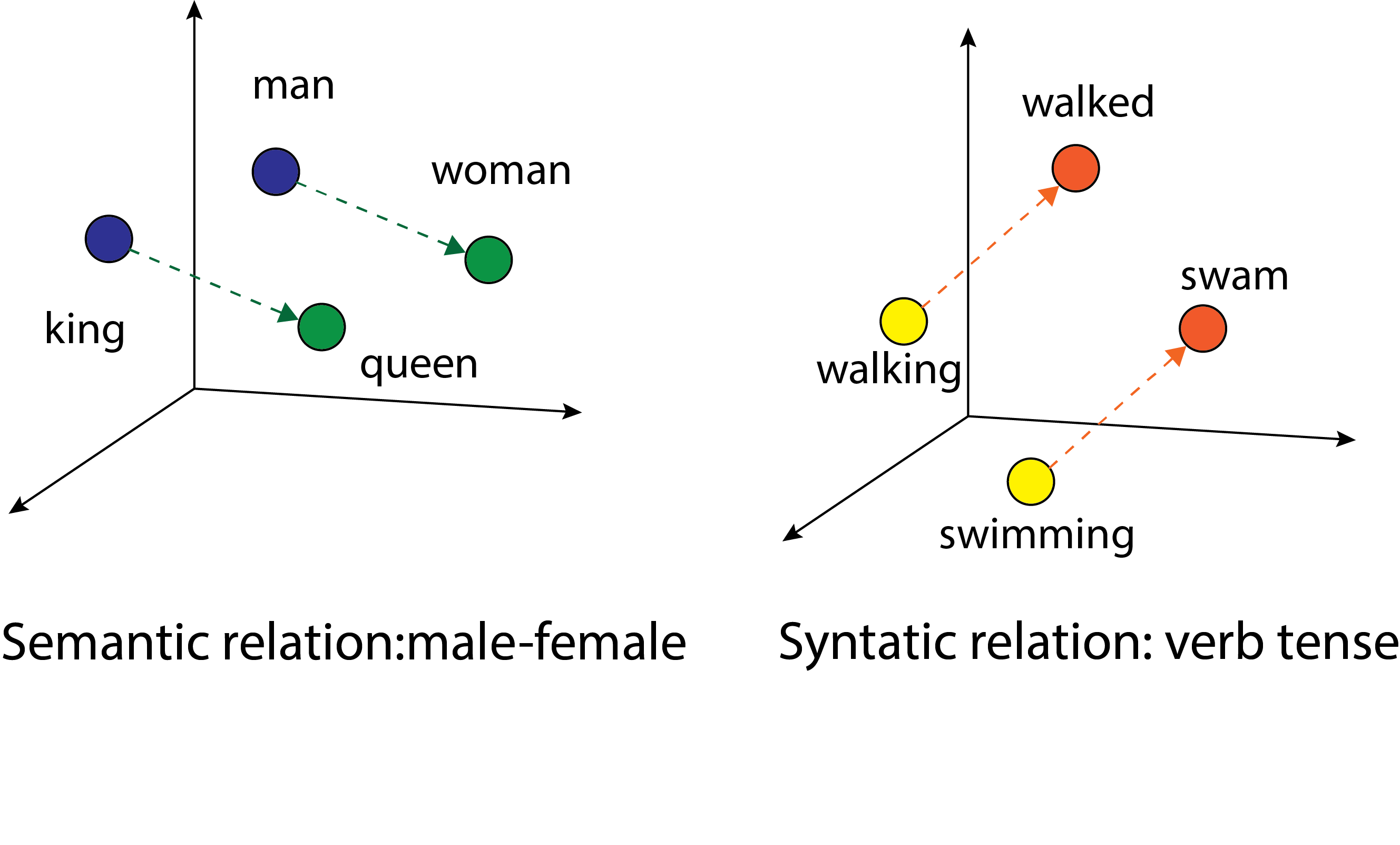
Fig. 4.1 (a) Embedding layer maps large, sparse one-hot vectors to short, dense vectors. (b) Example of low dimensional embeddings that capture semantic meanings.

In a dense vector representation, every component in the vector can contribute to enrich the concept and semantic meaning associated with the word. A linguistic phenomenon is that words that occur in similar contexts have similar meanings. Now the similarity or dissimilarity among words can be captured via distance in the vector space. A basic test on the ability to capture semantic and syntactic information is to be able to answer questions like

• Semantic questions like “Being is to China as Berlin is to [\(\cdot\)]”.

• Syntactic questions like “dance is to dancing as run is to [\(\cdot\)]”.

Ideally, we would like the word embeddings distributed in the vector space in certain way that capture semantic and syntactic relations and facilitates answering these questions.

There are different ways to obtain word embeddings. In the following sections, we will discuss methods that utilize classical singular value decomposition as well as modern neural network.

Table 4.1 Examples of five types of semantic relationships.

Type of relationship	Word Pair 1	Word Pair 1	Word Pair 2	Word Pair 2
Common capital city	Athens	Greece	Oslo	Norway
All capital cities	Astana	Kazakhstan	Harare	Zimbabwe
Currency	Angola	kwanza	Iran	rial
City-in-state	Chicago	Illinois	Stockton	California
Man-Woman	brother	sister	grandson	granddaughter

Table 4.2 Examples of nine types of syntactic relationships.

Type of relationship	Word Pair 1	Word Pair 1	Word Pair 2	Word Pair 2
Adjective to adverb	apparent	apparently	rapid	rapidly
Opposite	possibly	impossibly	ethical	unethical
Comparative	great	greater	tough	tougher
Superlative	easy	easiest	lucky	luckiest
Present Participle	think	thinking	read	reading
Nationality adjective	Switzerland	Swiss	Cambodia	Cambodian
Past tense	walking	walked	swimming	swam
Plural nouns	mouse	mice	dollar	dollars
Plural verbs	work	works	speak	speaks

4.2. SVD based word embeddings

Here we introduce a way to obtain low-dimensional representation of a word vector that capture the semantic and syntactic relation between words by performing SVD on a matrix constructed on a large corpus. The matrix used to perform SVD can be a co-occurrence matrix or it can be a document-term matrix, which describes the occurrences of terms in documents. When the matrix is the document-term matrix, this method is also known as latent semantic analysis (LSA)[Dum04].

Co-occurrence matrix is a big matrix whose entry encode the frequency of a pair of words occurring together within a fixed length context window. More formally, let \(M\) be a co-occurrence matrix, and we have

\[M_{ij} = \frac{\#(w_i, w_j)/n_{pair}}{\#(w_i)/n_{words}\cdot \#(w_j)/n_{words}}\]

where \(\#(w_i, w_j)\) is the number of co-occurrence of words \(w_i\) and \(w_j\) within a context window, \(n_{pair}\) is the total number pairs, \(n_{words}\) is the total number of words.

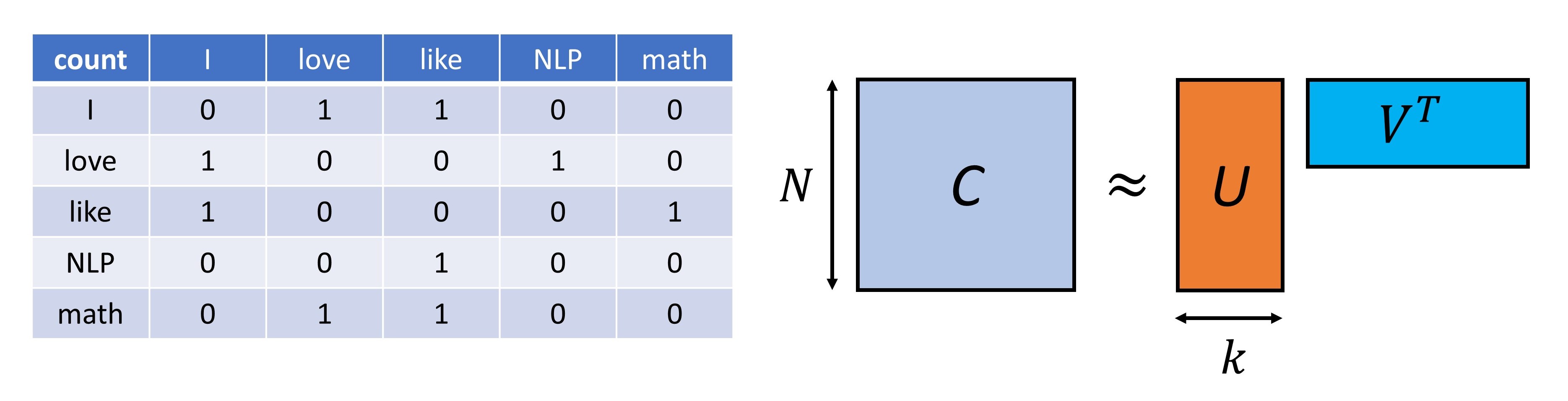
Fig. 4.2 (left) Example of co-occurrence matrix constructed from corpus “I love math” and “I like NLP”. The context window size of 2. (right) We can obtain lower-dimensional word embeddings from SVD truncated factorization of the co-occurrence matrix. Such low-dimensional embeddings captures important semantic and syntactic information in the co-occurrence matrix.

Another popular matrix to capture the co-occurrence information is the the pointwise mutual information (PMI) [ALL+16]. PMI entry for a word pair is defined as the probability of their co-occurrence divided by the probabilities of them appearing individually,

\[M^{PMI}_{ij} = \log \frac{p(w_i, w_j)}{p(w_i)p(w_j)} \approx \log M_{ij}.\]

The co-occurrence information captures to some extent both semantic and syntactic information. For example, terms tend to appear together either because they have related meanings (a semantic relationship, e.g., write and book) or because the grammar rule specifies so (a syntactic relation, e.g., verbs and to).

By using truncated SVD to decompose the co-occurrence matrix, we obtain the low-dimensional word vectors that preserve the co-occurrence information, or the semantic and syntactic relation implied by the co-occurrence information. For example, in the low-dimensional representation, apple and pear are expected to be closer (in terms of Euclidean distance of the embedding vector) than apple and dog.

More formally, via truncated SVD, we have factorization

\[M \approx UV^T\]

where \(M\in R^{N\times N}\), \(N\) is the size of the one-hot vector, \(U, V \in \mathbb{R}^{N\times k}, k << N\). Columns of \(U\) are the basis vector in latent word space. Each row in \(V\) is the low dimensional representation of a word in the latent word space.

The word embeddings derived from the co-occurrence matrix preserves semantic information within a relative local context window. For words that do not appear frequently within a context window but actually share semantic links, the word embeddings might miss the link.

This shortcoming can be overcome by performing a SVD on a document-term matrix. The document-term matrix is a sparse matrix whose rows correspond to terms and whose columns correspond to documents. The typical entry is the tf-idf (term frequency–inverse document frequency), whose value is proportional to frequency of the terms appear in each document, where common terms are downweighted to de-emphasize their relative importance.

A truncated SVD produces document vectors and term vectors (i.e., word embeddings). In constructing the document-term matrix, documents are just cohesive paragraphs covering one or multiple closely related topics. Words appear in a document therefore share certain semantic links. Overall, the decomposition results can be used to measure word-word, word-document and document-document relations. For example, document vector can also be used to measure similarities between documents.

4.3. Word2Vec

4.3.1. The model

In SVD based word embeddings, we introduce a SVD based matrix decomposition method to map one-hot word vector to semantic meaning preserving dense word vector. This section, we introduce a neural networ based method. The two classical methods, called continuous bags of words (CBOW)[MCCD13] and Skip-gram [MSC+13]. Both methods employ a three-layer neural networks [Fig. 4.3], taking a one-hot vector as input and predict the probability of its nearby words.

• In CBOW, the inputs are surrounding words within a context window of size \(c\) and the goal is to predict the central word (same as multi-class classification problems);

• In Skip-gram, the input is the single central word and the goal is to predict its surrounding words within a context window.

Denote a sequence of words \(w_1, w_2, ..., w_T\) (represented as integer indices) in a text, the objective of a Skip-gram model is to maximize the likelihood of observing the occurrence of its surrounding words within a context window of size \(c\), given by

\[\frac{1}{T} \sum_{t=1}^{T} \sum_{-c \leq j \leq c, j \neq 0} \log p\left(w_{t+j} | w_{t}\right)\]

where we have assumed conditional independence given word \(w_t\).

In the neural networks of Skip-gram and CBOW, we use Softmax function after the output layer to produce classification probability for \(V\) classes, where \(V\) is the size of the vocabulary. Note that the input layer has a weight matrix \(W\in \mathbb{R}^{V\times D}\) that performs look-up and converts a word integer to a dense vector of \(D\) dimension; the output layer has a weight matrix \(W'\in \mathbb{R}^{D\times V}\). The classification probability is given by

\[p(w_k|w_j) = \frac{\exp(v'_k\cdot v_j)}{\sum_{i=1}^V \exp(v'_i\cdot v_j)},\]

where \(v_i\) is the column \(i\) of the input matrix \(W\), and \(v'_i\) is the row \(i\) in the output matrix \(W'\).

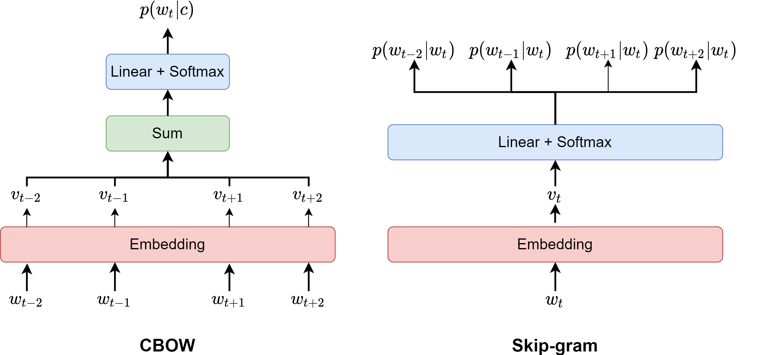
Fig. 4.3 (a) The CBOW architecture that predicts the central word given its surrounding context words. (b) The Skip-gram architecture that predicts surrounding words given the central word. The embedding layer is represented by a \(V\times D\) weight matrix that performs look-up for each word token integer index, where \(V\) is the vocabulary size and \(D\) is the dimensionality of the dense vector. The linear output layer is also represented by a \(V\times D\) weight matrix that is used to compute the logit for each token label as sort of classification over the vocabulary.

Definition 4.1 (Skip-gram and CBOW optimization problem)

The neural network weights \(\{v_i, v_i'\}\) of the Skip-Gram model are optimized to maximize the observation of a text consisting of words \(w_1, w_2, ..., w_T\), which can then be written by

\[\begin{split}\begin{align} & \max_{v,v'} \sum_{t = 1}^T\sum_{-c \leq j \leq c, j \neq 0} \ln p\left(w_{t+j} | w_{t}\right) \\ =&\max_{v,v'} \sum_{t=1}^{T} \sum_{-c \leq j \leq c, j \neq 0} \ln \frac{\exp \left(v^{\prime}_{t+j} \cdot v_{t)}\right)}{\sum_{w \in V} \exp \left(v_{w}^{\prime} \cdot v_{t}\right)} \\ =&\max_{v,v'} \sum_{t=1}^{T} \sum_{-c \leq j \leq c, j \neq 0}\left[v^{\prime}_{t+j} \cdot v_{t}-\ln \sum_{w \in V} \exp \left(v_{w}^{\prime} \cdot v_{t}\right)\right] \end{align} \end{split}\]

In the CBOW model, the optimization problem becomes

\[\begin{split} \begin{align} &\max_{v,v'} \sum_{t = 1}^T \ln p\left(w_{t} | w_{t-c}, ..., w_{t+c}\right) \\ =&\max_{v,v'} \sum_{t=1}^{T} \ln \frac{\exp(v'_t \cdot \sum_{-c \leq j \leq c, j \neq 0} v_j)}{\sum_{i=1}^V\exp(v'_i \cdot \sum_{-c \leq j \leq c, j \neq 0} v_j)} \end{align} \end{split}\]

In the original Skip-gram and the CBOW model, each word will have two embeddings, \(v_i\) and \(v_i'\) in the input matrix \(W\) and the output matrix \(W'\), respectively. Notable, the embedding \(v_i'\) corresponds to the dense word vector that produces one-hot probability vector in the output. For these two embeddings, we can use one of them, a mixed version of them, and a concatenated one. It is only found that tying the two weight matrices together can lead to performance [IKS16, PW16].

With the trained embeddings for each word, we can assemble then into a matrix of size \(D\times V\), which is also called an Embedding layer. In applications, the one-hot word vector is fed into the embedding layer and produce the corresponding dense word vectors. From the computational perspective, we do not need to perform matrix multiplication; instead, we can view the Embedding layer as a dictionary that maps integer indices of the word to dense vectors.

Remark 4.1 ((Skip-gram vs CBOW performance))

In Skip-gram, the weight associated with each word receives adjustment signal (via gradient descent) from its surrounding context words. In CBOW, a central word provides signal to optimize the weights of its multiple surrounding words. Skip-gram is more computational expensive than CBOW as the Skip-gram model has to make predictions of size \(O(cV)\) while CBOW makes prediction on the scale of \(O(V)\). Further, because of the averaging effect from input layer to hidden layer in CBOW, CBOW is less competent in calculating effective word embedding for rare words than Skip-gram.

4.3.2. Optimization I: negative sampling

Solving Skip-gram optimization [Definition 4.1] requires summing over the probabilities of every incorrect vocabulary word in the denominator (\(\sum_{w \in V} \exp \left(v_{w}^{\prime} \cdot v_{t}\right)\)). In a practical scenario, the dimensionality of the word embedding \(D\) could be \(\sim 500\) and the size of the vocabulary \(|V|\) could be \(\sim 10,000\). Naively running gradient descent on the optimization would lead to update millions of network weight parameters (\(O(D|V|)\)). Computing the summation is therefore costly. One idea to reduce the cost is: just summing over probabilities of a few (e.g., \(k = 5\sim 20\) for small corpus and \(k=2\sim 5\) for large-scale corpus) high-frequent incorrect words, rather than summing over the probabilities of every incorrect word. These chosen non-target words are called negative samples. Note that negative sampling will result in incorrect normalization since we are not summing over the vast majority of the vocabulary. In practice, this approximation that turns out to work well. Further, the computational cost to update weight parameters goes from \(O(D\cdot |V|)\) to \(O(D\cdot k)\).

In the optimization, gradient descent steps tend to pull embeddings of frequently co-occurring words closer (i.e., to make \(v_i\cdot v_j\) have a larger value) while push embeddings of rarely co-occurring words away (i.e., to make \(v_i\cdot v_j\) have a smaller value). Because frequent words are more frequently used as positive examples, it is justified to pick more commonly seen words with larger probability as negative samples to compensate. This is similar to the idea of hard negative mining in contrastive learning. In this way, embeddings of commonly seen words will be encouraged to stay away from other commonly seen but irrelevant words. In the study, the negative samples \(w\) are empirically sampled from

\[P_n(w) = \frac{f(w)^{3/4}}{\sum_{w'\in V} f(w')^{3/4}},\]

where \(f(w)\) is the frequency of word \(w\) in the training corpus, and \(P_n(w)\) is a montonic function on \(w\). This distribution is found to significantly outperform uniform distribution [MSC+13].

Finally, we have the modified optimization for Skip-gram model given by

\[\operatorname{argmax}_{v,v'} \sum_{t=1}^{T} \sum_{-c \leq j \leq c, j \neq 0}\left[v^{\prime}_{t+j} \cdot v_{t}-\log \sum_{m=1}^k \exp \left(v_{w_m}^{\prime} \cdot v_{t}\right)\right] \]

where \(w_m \sim P_n(w), m=1,...,k\) are negative samples.

4.3.3. Optimization II: down-sampling of frequent words

In very large corpora, the most frequent words can easily occur hundreds of millions of times (e.g., in, the, and a). These words usually provide less information value than the rare words. For example, while the Skip-gram model gains more information from observing the co-occurrences of China and Beijing, it gains much less information from observing the frequent co-occurrences of France and the, as nearly every word co-occurs frequently within a sentence with the. More importantly, as the model is pushing embeddings of co-occurring words closer, it might lead to the case that most words are quite close to these frequent words.

Therefore, we like to reduce the sampling probability for these frequent words when constructing training samples. This is achieved via a simple down-sampling approach: each word \(w_{i}\) in the training set is discarded with probability computed by the formula

\[ P\left(w_{i}\right)\approx1-\sqrt{\frac{t}{f\left(w_{i}\right)}} \]

where \(f(w_i)\) is the frequency of word \(w_i\) and \(t\) is a chosen threshold, typically around \(10^{-5}\). Clearly, the larger the frequency of a word, the larger the probability of being discarded.

4.3.4. Noise Contrastive Estimation

An alternative approach to the above sampled Softmax loss formulation is using Noise Contrastive Estimation (NCE). NCE can be viewed as an optimization based on binary classification using logistic regression [GL14] that ranks observed data above noise. The class labels are positive pairs, which are formed by each word and the word in its context windows, and negative pairs, which are formed by each word and negatively sampled words. NCE can be shown to approximately maximize the log probability of the Softmax [CW08].

Denote \(D\) as the set of positive pairs with label \(y=1\) and \(D'\) the set of negative pairs with label \(y=0\). The NCE formulation minimize the following binary cross-entropy given by

\[\begin{split} \begin{align} & \operatorname{argmin}_{\theta} -\left(\sum_{(w, c) \in D\cup D'} y\log \sigma\left(v_{c} \cdot v_{w}\right)+ (1 - y) \log \sigma\left(-v_{c} \cdot v_{w}\right)\right) \\ & \operatorname{argmin}_{\theta} -\sum_{(w, c) \in D} \log \sigma\left(v_{c} \cdot v_{w}\right)-\sum_{(w, c) \in D^{\prime}} \log \sigma\left(-v_{c} \cdot v_{w}\right) \end{align} \end{split}\]

4.3.5. Limitations and Challenges

Word2Vec was a revolutionary word embedding technique that represents words as numerical vectors, capturing semantic relationships between them. However, it also have some limitations.

Out-of-Vocabulary (OOV) words: One of the most significant limitations of Word2Vec, is its inability to handle words it hasn’t seen during training. When the model encounters an OOV word, it cannot create a meaningful vector for it.

Lack of sub-word level understanding: Word2Vec treats each word as a distinct unit, disregarding any sub-word level information. This can be a major drawback, especially for languages with rich morphology, where words have complex structures and inflections. For example, the model may not accurately capture the relationship between “play,” “playing,” and “played.” This limitation can hinder the model’s ability to understand the nuances of language and affect its performance in tasks like machine translation or text generation.

Difficulty in handling polysemy: Polysemy refers to the phenomenon where a single word has multiple meanings (e.g., bank in financial banking vs river bank). Word2Vec assigns a single vector to each word, irrespective of its different senses.

Limited contextual understanding: While Word2Vec considers the surrounding words of a target word, it often struggles to capture the broader context of a sentence or document. This is because only a limited context window is used in constructing training data, which may not be sufficient to capture long-range dependencies and complex relationships between words.

Insensitive to word order: Word2Vec models do not fully capture the nuances of word order. Word order information is not considered in both the Skip-gram and the CBOW model loss function.

Rare words: While the Skip-gram model is generally better at handling infrequent words than the CBOW model , it may still struggle to create accurate representations for rare words if the training data is limited.

4.3.6. Visualization

We can visualize the word embedding space by projecting onto a 2D plane using two leading principal components [Fig. 4.4]. The neighboring words of apple include macintosh, microsoft, ibm, Windows, mac, intel, computers as well as wine, juice, which capture to some extent the two common meanings in the word apple. This example also reveals the drawback of the word2vec approach in representing multi-meaning words (known as polysemy), where we associate each token with a fixed/static embedding irrespective of context. For example, apple in I like to eat an apple vs Apple is great company means two different things and have the same embedding.

Another example is the word bank, which has two contrasting meanings in the following two sentences:

• We went to the river bank.

• I need to go to bank to make a deposit.

The nearest words of bank in the Word2Vec model are banks, monetary, banking, imf, fund, currency, etc. , which does not capture the second meaning. More formally, we say static word embeddings from Word2Vec model cannot address polysemy.\footnote{the coexistence of many possible meanings for a word or phrase.} On the other hand, the mean of a word can usually be inferred from its left and right context. Therefore it is also essential to develop context-dependent embeddings, which will be discussed in BERT.

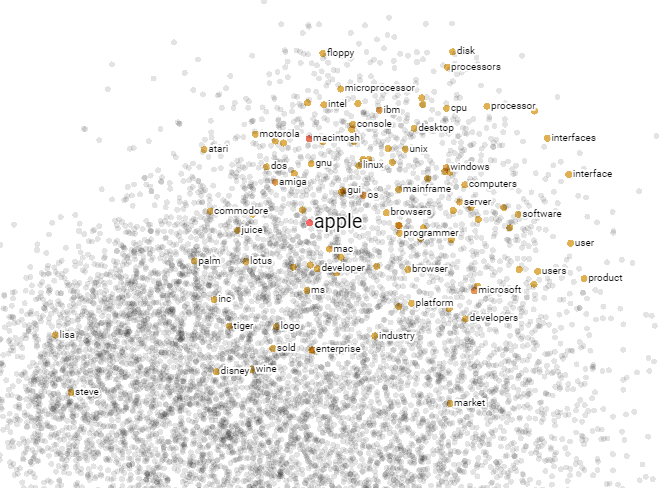
Fig. 4.4 Visualization of neighboring words of apple in a 2D low-dimensional space (first two components via PCA). Image from Tensorflow projector (https://projector.tensorflow.org/).

4.4. GloVe

4.5. Subword model

The word embedding models we discussed so far are typically trained on a large corpus. On the runtime inference stage, there is no guarantee that the words we see during the runtime are in the vocabulary of the training corpus. Those words are known of out-of-vocabulary words, OOV words. Another issue with previous word embedding models is that some text normalization techniques \footnote{Some typical text normalization include contraction expansion, stemming, lemmatization, etc. For example, in contraction expansion, we have ain’t \(\to\) are not. Lemmatization is to reduce words to their base forms.} are performed to standardize texts. While text normalization allows statistics and parameter sharing across words of the same root (e.g., bag and bags) and save computational memory and cost, it also ignores meanings that could be encoded in these morphological variations.

Facebook AI research [BGJM17] proposed a key idea that one can derive word embeddings by aggregating sub-word level embeddings. It has several advantages: First it addresses the OOV problem by breaking down uncommon words into subword units that are in the training corpus. For example, for the gregarious that’s not found in the embedding’s word vocabulary, we can break it into following character 3-grams, gre, reg, ega, gar,rio, iou, ous and combine embeddings of these n-grams to arrive at the embedding of gregarious. Second, this approach enables modeling morphological structures (e.g., prefixes, suffixes, word endings, etc.) across words. For example, dog, dogs and dogcatcher have the same root dog, but different suffixes to modify the meaning of the word. By allowing parameter sharing across subword units, the eventual word vectors will be enriched with subword level information.

Such subword level modeling is posing an inductive bias that words with similar subword components tend to share similar meaning. For example, the similarity between dog and dogs are directly expressed in the model. On the other hand, in CBOW or Skip-gram, they are either treated as two different vectors and the same vector, depending on the text normalization applied in the pre-processing step.

The subword model follows the same optimization framework of Skip-gram. Denote a sequence of words \(w_1, w_2, ..., w_T\) (represented as integer indices) in a text, the objective of a Skip-gram model is to maximize the likelihood of observing the occurrence of its surrounding words within a context window of size \(c\), given by

\[\frac{1}{T} \sum_{t=1}^{T} \sum_{-c \leq j \leq c, j \neq 0} \log p\left(w_{t+j} | w_{t}\right),\]

where we have assumed conditional independence given word \(w_t\). Further applying the negative sampling technique [Noise Contrastive Estimation], we arrive at the approximate loss function given by

\[\begin{split} \begin{align*} L &= - \sum_{t=1}^T \left(\log \sigma(s(w_t,w_c)) + \sum_{n \in \mathcal{N}_{t, c}} \log \sigma(-s(w_t, n))\right) \\ & =- \sum_{t=1}^T \left(\log \left(1+e^{-s\left(w_{t}, w_{c}\right)}\right)+\sum_{n \in \mathcal{N}_{t, c}} \log \left(1+e^{s\left(w_{t}, n\right)}\right)\right). \end{align*}\end{split}\]

Here the score function is computed via \(s(w_t, w_c) = v_t' \cdot v_c\), where \(v_t'\) is the word vector in the input layer and \(v_c\) is the word vector in the output layer.

In the subword model, Each word \(w\) is represented as a bag of character \(n\)-gram. Word boundary symbols \(<\) and \(>\) are dded at the beginning and end of words to distinguish prefixes and suffixes from other character sequences. For example, the word where will be presented as by 3-grams of <wh, whe, her, ere, re>

In the subword model, we have a vocabulary \(V\) of regular words as well as a vocabulary of \(n\)-grams of size \(G\). Given a word \(w,\) whose \(n\)-gram decomposition is \(\mathcal{G}_{w} \subset\{1, \ldots, G\}\), we let the embedding of \(w\) be the sum of the vector representations of its \(n\) -grams. That is

\[v_w = \sum_{g \in \mathcal{G}_{w}} {z}_{g}^{\top}, \]

where \({z}_{g}\) is the vector representation of \(n\)-gram \(g\).

We goal in the training phase is to learn \(z_g\), which can be realized by using the skip-gram optimization except that the scoring function is now

\[ s(w, c)=\sum_{g \in \mathcal{G}_{w}} {z}_{g}^{\top} {v}_{c}, \]

where \(v_c\) is the column vector in the output layer matrix associated with word \(c\).

After the \(n\)-gram embeddings are trained, we can compute word embedding of each word by aggregating its constituent \(n\)-gram embeddings.

Note that the vocabulary size of \(G\) can be huge for large \(n\). Below is the maximum number of \(n\) -grams as a function of \(n\).

n-grams	maximum number of subwords
3	17576
4	26^4 ≈ 4.6×10^5
5	26^5 ≈ 1.2×10^7
6	26^6 ≈ 3.1×10^8

In order to bound the model memory requirements, we can use a hashing function that maps \(n\) -grams to \(K\) (e.g., \(K \approx 10^6\)) buckets. Note that when collison occurs, two \(n\)-grams will share the same embedding.

One direct application of subword representation is the Fasttext text classifier [JGBM16], which use subword embedding as the feature in the logistic regression model.

4.6. Bibliography

[ALL+16]

Sanjeev Arora, Yuanzhi Li, Yingyu Liang, Tengyu Ma, and Andrej Risteski. A latent variable model approach to pmi-based word embeddings. Transactions of the Association for Computational Linguistics, 4:385–399, 2016.

[BGJM17]

Piotr Bojanowski, Edouard Grave, Armand Joulin, and Tomas Mikolov. Enriching word vectors with subword information. Transactions of the Association for Computational Linguistics, 5:135–146, 2017.

[CW08]

Ronan Collobert and Jason Weston. A unified architecture for natural language processing: deep neural networks with multitask learning. In Proceedings of the 25th international conference on Machine learning, 160–167. 2008.

[Dum04]

Susan T Dumais. Latent semantic analysis. Annual review of information science and technology, 38(1):188–230, 2004.

[GL14]

Yoav Goldberg and Omer Levy. Word2vec explained: deriving mikolov et al.'s negative-sampling word-embedding method. arXiv preprint arXiv:1402.3722, 2014.

[IKS16]

Hakan Inan, Khashayar Khosravi, and Richard Socher. Tying word vectors and word classifiers: a loss framework for language modeling. arXiv preprint arXiv:1611.01462, 2016.

[JGBM16]

Armand Joulin, Edouard Grave, Piotr Bojanowski, and Tomas Mikolov. Bag of tricks for efficient text classification. arXiv preprint arXiv:1607.01759, 2016.

[MCCD13]

Tomas Mikolov, Kai Chen, Greg Corrado, and Jeffrey Dean. Efficient estimation of word representations in vector space. arXiv preprint arXiv:1301.3781, 2013.

[MSC+13] (1,2)

Tomas Mikolov, Ilya Sutskever, Kai Chen, Greg S Corrado, and Jeff Dean. Distributed representations of words and phrases and their compositionality. In Advances in neural information processing systems, 3111–3119. 2013.

[PW16]

Ofir Press and Lior Wolf. Using the output embedding to improve language models. arXiv preprint arXiv:1608.05859, 2016.