6. BERT

6.1. Contextual Embedding

In natural language processing, although we have seen many successful end-to-end systems , they usually require large scale training examples and the systems require a complete retrain for a different task. Alternatively, we can first learn a good representation of word sequences that not task-specific but would be likely to facilitate downstream specific tasks. Learning a good representation in prior from broadly available unlabeled data also resembles how human perform various intelligent tasks. In the context of natural languages, a good representation should capture the implicit linguistic rules, semantic meaning, syntactic structures, and even basic knowledge implied by the text data.

With a good representation, the downstream tasks can be significantly sped up by fining tuning the system on top of the representation. Therefore, the process of a learning a good representation from unlabeled data is also known as pre-training a language model.

Pre-training language models have several advantages:

• first, it enable the learning of universal language representations that suit different downstream tasks;

• second, it usually gives better performance in the downstream tasks after fine-tuning on a target task;

• finally, we can also interpret pre-training as a way of regularization to avoid overfitting on small data set.

In Word Embeddings, we discussed different approaches (e.g., Word2Vec, GloVe) to learning a low-dimensional dense vector representation of word tokens. One significant drawback of these representations is context-independent or context-free static embedding, meaning the embedding of a word token is fixed no matter the context it is in. By contrast, in natural language, the meaning of a word is usually context-dependent. For example, in sentences I like to have an apple since I am thirty vs. I like to have an Apple to watch fun movies, the word apple mean the fruit apple and the electronic device, respectively.

There has been significant efforts directed to learning contextual embedding of word sequences[LKB20, QSX+20]. A contextual embedding encoder usually operates at the sequence level. As shown in the following, given a non-contextual word embedding sequence \(x_{1}, x_{2}, \cdots, x_{T}\), the contextual embeddings of the whole sequence are obtained simultaneously via $\(\left[{h}_{1}, {h}_{2}, \cdots, {h}_{T}\right]=\operatorname{ContextualEncoder}\left(x_{1}, x_{2}, \cdots, x_{T}\right).\)$

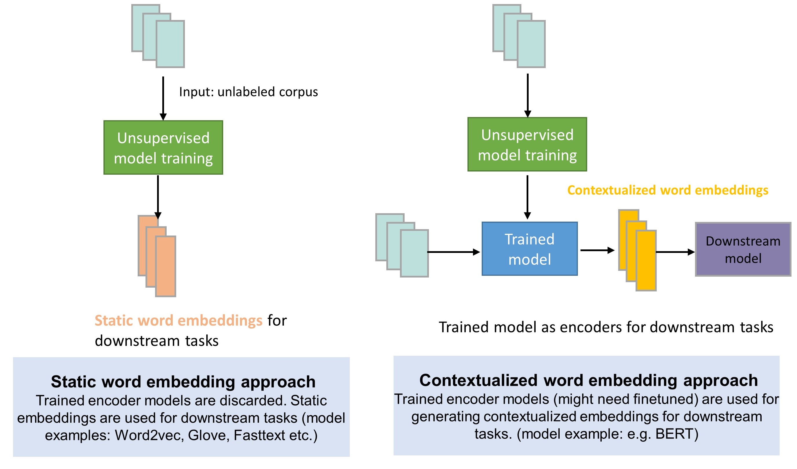
Fig. 6.1 Static word embedding approach vs. contextualized word embedding approach.

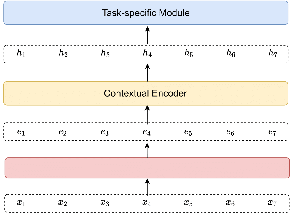
Fig. 6.2 A generic neural contextual embedding encoder.

Given large-scale unlabeled data, the most common way to learn a good representation is via self-Supervised learning. The key idea of self-Supervised learning is to predict part of the input from other parts in some form (e.g., add distortion). By minimizing prediction task loss or other auxiliary task losses, the neural network learns good presentations that can be used to speed up downstream tasks.

Since the advent of the most successful pretrained language model BERT [DCLT18], many follow-up research found that the performance of the pretrained model in downstream tasks highly depend on the self-supervised tasks in the pretraining stage. If the downstream tasks are closely related to self-supervised tasks, a pretrained model can offer significant performance boost. And the fine tuning process can be understood as a process that further improves features relevant to downstream tasks and discards irrelevant features.

6.2. BERT Architecture Componenents

BERT, Bidirectional Encoder Representations from Transformers [DCLT18], is one of the most successful pre-trained language model. BERT relies on a Transformer (the attention mechanism that learns contextual relationships between words in a text). BERT model heavily utilizes stacked self-attention modules to contextualize word embeddings.

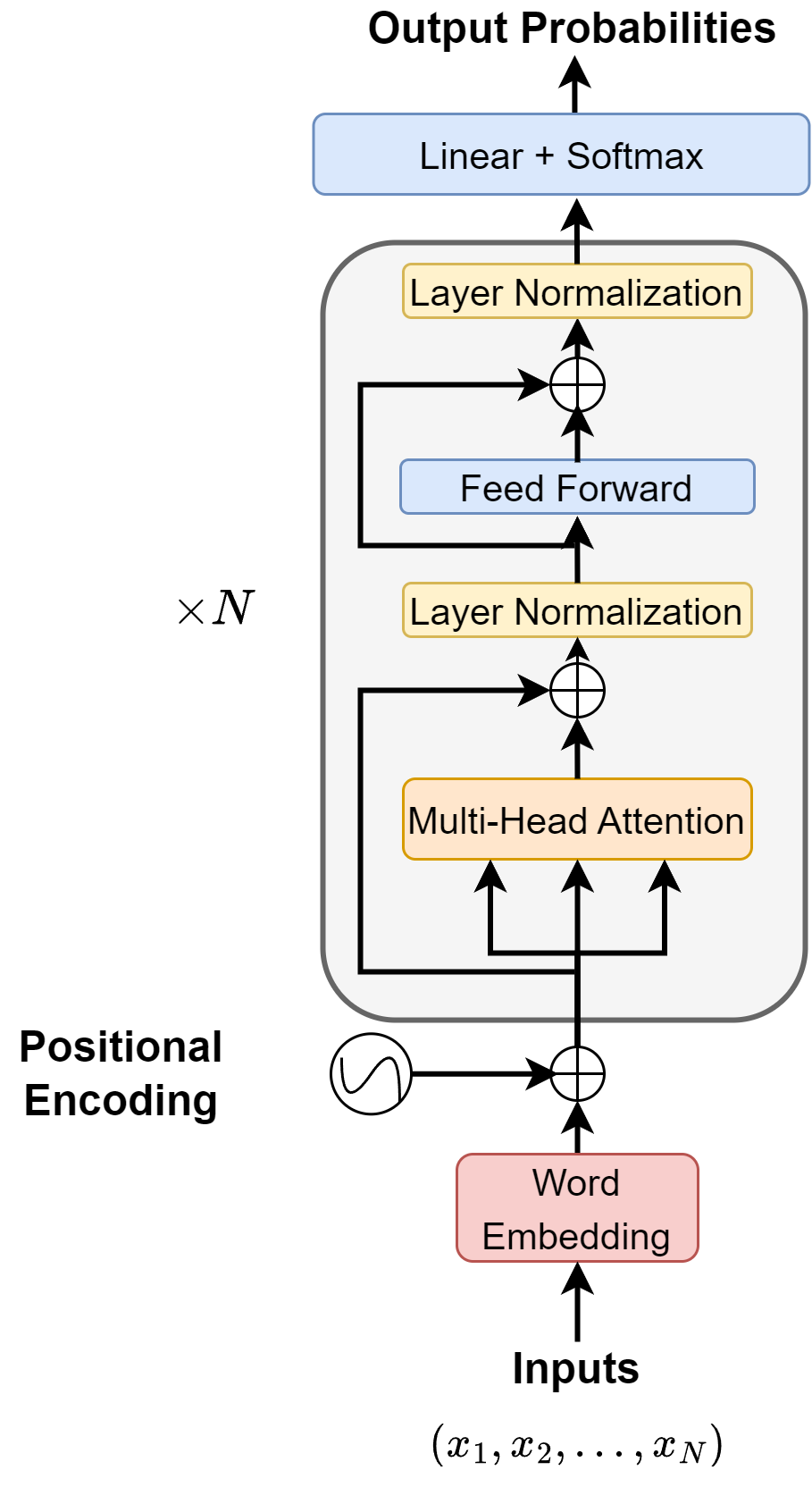
Fig. 6.3 BERT model architecture.

In the following, we will go through detailed structure of BERT.

6.2.1. Input Embeddings

The input to the BERT is a sequence of token representations. The representation of each token is a dense vector of dimensionality \(d_{model}\), which is the summation of following components:

• Token embedding of dimensionality \(d_{model}\), which is the ordinary dense word embedding. Specifically, a sub-word type of embedding, called wordPiece embedding [WSC+16], with a 30,000 token vocabulary is used. Note that A [CLS] token is added to the input word tokens at the beginning of the first sentence and a [SEP] token is inserted at the end of each sentence.

• Segment embedding of dimensionality \(d_{model}\), which is a marker 0 or 1 indicating if sentence A precedes sentence B. Segment embedding is typically learned from the training.

• Positional embedding of dimensionality \(d_{model}\), which encodes information of position in the sentence. Positions matters in word and sentence level meanings. For example, I love you and you love me are different. Position embedding is a vector depending on where the token is located in the segment. It is a constant vector throughout the training. See Position Encodings on how typical absolute position encoding is constructed.

The token, segment, and position embeddings are implemented through a look-up matrix. The token embedding look-up matrix has a size of \((vocab~size, d_{model})\); the position embedding look-up matrix has a size of \((max~len, d_{model})\); the segment embedding look-up matrix has a size of \((2, d_{model})\).

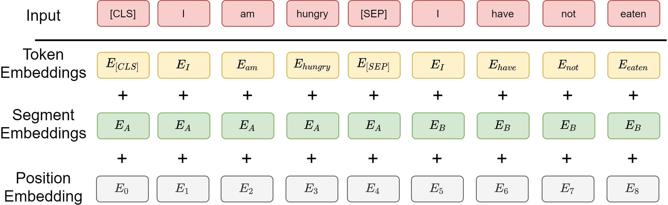
Fig. 6.4 Input embedding in BERT, which consists of token embedding, segmenet embedding and positional embedding.

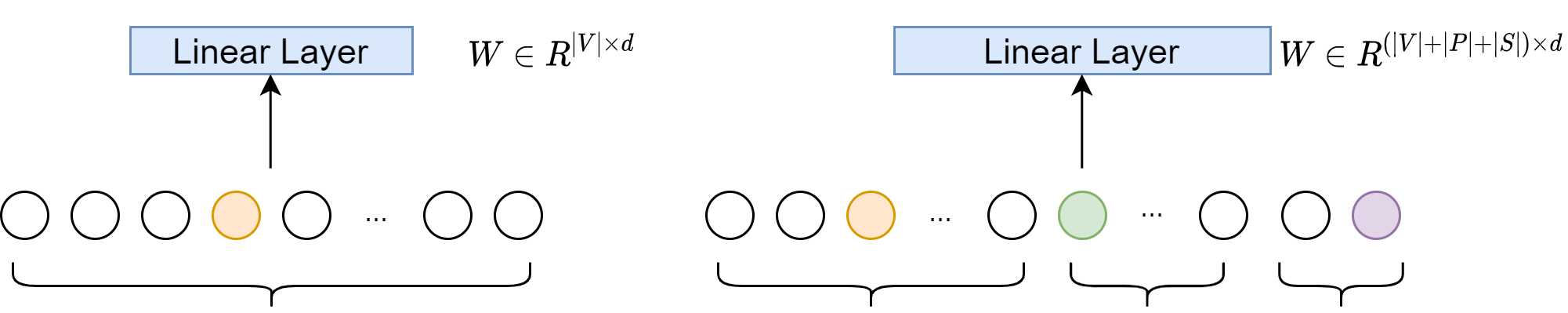
Fig. 6.5 Embedding layer interpretation.

The addition of token embedding, segment embedding, and position embedding for for each token can be viewed as feature fusion via concatenation of one-hot vectors \((O_{\text {tok }}, O_{\text {seg }}, O_{p o s})\). The resulting feature vector is given by

\[\begin{split} E_{\text {word }}=\left[\begin{array}{lll} O_{\text {tok }} & O_{\text {seg }} & O_{p o s} \end{array}\right]\left[\begin{array}{c} W_{t o k}^{|V| \times H} \\ W_{s e g}^{|S| \times H} \\ W_{p o s}^{|P| \times H} \end{array}\right]. \end{split}\]

6.2.2. The Encoder Anatomy

Following the detailed description of Transformer architecture in Overall Architecture, here we summarize the computations happen within each of the BERT Encoder layer.

Definition 6.1 (Encoder layer)

:label: chapter_foundation_def_pretrained_LM_transformer_bert_encoder_layer

The BERT encoder with \(n\) sequential inputs can be decomposed into following calculation procedures

\[\begin{split}\begin{align} e_{mid} &= \operatorname{LayerNorm} (e_{in} + \operatorname{MultiHeadAttention}(e_{in}, e_{in}, e_{in}, padMask)) \\ e_{out} &= \operatorname{LayerNorm} (e_{mid} + \operatorname{FFN}(e_{mid})) \end{align} \end{split}\]

where \(e_{mid}, e_{out} \in \mathbb{R}^{n\times d_{model}}, \)

\[\operatorname{FFN}(e_{mid}) = \max(0, e_{mid} W_1 + b_1)W_2 + b_2,\]

with \(W_1\in \mathbb{R}^{d_{model}\times d_{ff}}, W_2\in \mathbb{R}^{d_{ff}\times d_{model}}, b_1 \in \mathbb{R}^{d_{ff}}, b_2\in \mathbb{R}^{d_{model}}\), and the \(padMask\) excludes padding symbols in the sequence.

In a typical setting, we may have \(d_{\text {model }}=512\), and the inner-layer has dimensionality \(d_{f f}=2048\). Also note that there is active research on where to optimally add the layer normalization in the encoder.

The whole computation in the encoder module can be summarized in the following.

Definition 6.2 (computation in encoder module)

Given an input sequence represented by integer sequence \(s = (i_1,...,i_p,...,i_n)\) and its position \(s^p = (1,..., p, ..., n)\). The encoder module takes \(s, s^p\) as inputs and produce \(e_N \in \mathbb{R}^{n\times d_{model}}\).

\[\begin{split}\begin{align} e_{0}&=\operatorname{WE}(s)+ \operatorname{PE}(s^p) \\ e_1 & = \operatorname{EncoderLayer}(e_0) \\ e_2 & = \operatorname{EncoderLayer}(e_1) \\ &\cdots \\ e_L & = \operatorname{EncoderLayer}(e_{L - 1}) \end{align} \end{split}\]

where \(e_i \in \mathbb{R}^{n\times d_{model}}\), \(\operatorname{EncoderLalyer}: \mathbb{R}^{n\times d_{model}}\to \mathbb{R}^{n\times d_{model}}\) is an encoder sub-unit, \(N\) is the number of encoder layers. Specifically, this encoder layer is given by BERT model architecture.. Note that Dropout operations are not shown above. Dropouts are applied after initial embeddings \(e_0\), every self-attention output, and every point-wise feed-forward network output.

Note that Dropout operations are not shown above. Dropouts are applied after initial embeddings \(e_0\), every self-attention output, and every point-wise feed-forward network output.

Commonly used BERT models take the following configurations:

• BERT-BASE, \(L=12, d_{model}=768, H=12\), total Parameters 110M.

• BERT-LARGE, \(L=24, d_{model} = 1024, H=16\), total parameters 340M.

Table 6.1 The hyperparameter settings of various pretrained BERT configurations. BERTBase and BERTLarge are the two most commonly used configurations today;

Size	Layers	Hidden Size	Attention Heads	Parameters
Tiny	2	128	2	4 M
Mini	4	256	4	11 M
Small	4	512	4	29 M
Medium	8	512	8	42 M
Base	12	768	12	110 M
Large	24	1024	16	340 M

6.2.3. Compared with ELMO

An influential contextualized word embedding model via deep learning is ELMO (Embeddings from Language Models) [PNI+18], in which word vectors are learned functions of the internal states of a deep bidirectional LSTM language model [Fig. 6.6]. Given a sequence of \(N\) tokens (character-based), \(\left(t_{1}, t_{2}, \ldots, t_{N}\right)\). Their static word embeddings \((e_1,...,e_N)\) are contextualized by stacked bidirectional LSTM as \((h_1,...,h_N)\).

The LSTMs are pre-trained to perform language modeling task, i.e., predicting the next token given preceding tokens in forward and backward directions, respectively. Specifically, an linear plus Softmax layer take LSTM hidden states (two directions) as the input and computes the distribution. The following log-likelihood of the forward and backward directions is maximized:

\[ \sum_{k=1}^{N}\left(\log p\left(t_{k} \mid t_{1}, \ldots, t_{k-1} ;\Theta\right) +\log p\left(t_{k} \mid t_{k+1}, \ldots, t_{N} ; \Theta\right)\right)\]

After pretraining, the top layer LSTM hidden states are used as contextualized embeddings.

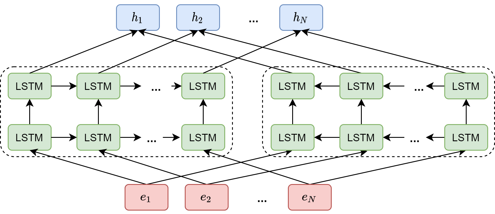
Fig. 6.6 In ELMO, static word embeddings \((e_1,...,e_N)\) are contextualized by stacked bidirectional LSTM as \((h_1,...,h_N)\).

Compared to ELMO, BERT is deeply bidirectional due to its novel masked language modeling technique. Having bidirectional context is expected to generate more accurate word representations.

Another improve of BERT over EMLO is the tokenization strategy. BERT tokenizes words into sub-words (using WordPiece), while ELMO uses character based input. It’s often observed that character level language models don’t perform as well as word based or sub-word based models.

6.2.4. Pre-training Tasks

6.2.4.1. Masked Language Modeling (Masked LM)

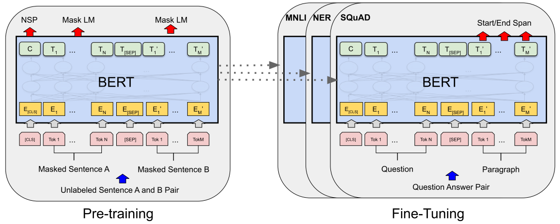
Fig. 6.7 BERT pre-training and downstream task fine tuning framework. Image from [DCLT18].

There are two tasks to pretrain the network: masked language modeling (Masked LM) and next sentence prediction (NSP).

In the Masked LM, some percentage of randomly sampled words in a sequence are masked, i.e., being replaced by a [MASK] token. The task is to predict (via Softmax) only the masked words, based on the context provided by the other non-masked words in the sequence.

Masked LM task has this drawback of introducing mismatch between the pre-training task and fine-tuning tasks: in the fine-tuning stage, training sentences do not contain masked tokens. To reduce the mismatch between pre-training and fine-tuning, different masking strategies are explored. It is found one effective strategy is to select 15% of tokens for the following possible replacement. For each token among the 15% selected tokens,

• 80% probability is replaced by [MASK].

• 10% probability is replaced by a random token.

• 10% probability is left unchanged.

The rationale for this masking strategy is that this forces the model to predict a word without relying on the word at the current position, since the word at the current position only has 10% probability of being correct. As such, the model adapts to make predictions based on contextual information, which helps the model to build up some error correction capability.

Formally, let \(\mathbf{x}=(x_1,...,x_T)\) be the original input and \(\hat{\mathbf{x}}\) be the masked noise input. The masked LM task aims to minimize the following negative log loss on masked tokens, which is given by

\[\min_{\theta} - \sum_{t=1}^{T} m_{t} \log p\left(x_{t} \mid \hat{\mathbf{x}}\right)=\sum_{t=1}^{T} m_{t} \log \frac{\exp \left(h_{t}^{T} e\left(x_{t}\right)\right)}{\sum_{x_{t'}} \exp \left(h_{t'}^{T} e\left(x_{t'}\right)\right)}\]

where \(m_t \in \{0, 1\}\) indicates if \(x_t\) is a mask token, \((h_1,...,h_T)\) are contextualized encodings produced by the encoder, \(e(x_t)\) is the weight vector (corresponding to token \(x_t\) in the vocabulary) in the prediction head, which consists of a linear layer and Softmax function.

Remark 6.1 (Imperfections of the masking strategy.)

• This masked LM task suffers from training inefficiency and slow convergence since each batch only 15% of masked tokens are predicted.

• The masked LM task is making conditional independence assumption. When we predict the masked tokens, we are assuming that different masked tokens are independent conditioning on masked input sequence.

  • For example, suppose the original sentence New York is a city and we mask the New and York two tokens. In our prediction, we assume these two masked tokens are independent, but actually New York is an entity that co-occur frequently. However, it should be noted that this conditional-independence assumption problem has not been a big in practice since the model is often trained on huge corpus to learn the inter-dependencies of these words.

  • This conditional independence assumption also make mask LM task not aligned with language generation tasks, in which predicted tokens are dependent on preceding tokens.

• Another drawback is that the mask can be applied to a sub-word piece due to fine-grained WordPieces tokenizer. For example, the word probability is tokenized into three parts: pro, #babi, and #lity. One might randomly mask #babi alone. In this case, the model can leverage the word spelling itself for prediction rather than the semantic context.

6.2.4.2. Next Sentence Prediction (NSP)

In the NSP, the network is trained to understand relationship between two sentences. A pre-trained model with this kind of understanding is relevant for tasks like question answering and natural language Inference. This task is also reminiscent of human language study exercise, where the learner needs to restore the correct order of sentences in a paragraph consisting of randomly displaced sentences.

The input for NSP is a pair of segments, which can each contain multiple natural sentences, but the total combined length must be less than 512 tokens. Notably, it is found that using individual natural sentence pairs hurts performance on downstream tasks[LOG+19].

The model is trained to predict if the second sentence is the next sentence in the original text. In choosing the sentences pair for each pretraining example, \(50 \%\) of the time, the second sentence is the actual next sentence of the first one, and \(50 \%\) of the time, it is a random sentence from the corpus.

The next sentence prediction task can be illustrated in the following examples.
Input: [CLS] the man went to [MASK] store [SEP] he bought a gallon [MASK] milk [SEP]
Label: IsNext
Input: [CLS] the man [MASK] to the store [SEP] penguin [MASK] are flight1ess birds [SEP] \ Label: NotNext

6.2.4.3. Put It Together

The pre-training is performed in a joint manner with loss function given by

\[ L\left(\theta, \theta_{1}, \theta_{2}\right)=\underbrace{L_{1}\left(\theta, \theta_{1}\right)}_{\text{Masked LM}}+\underbrace{L_{2}\left(\theta, \theta_{2}\right)}_{\text{NSP}}, \]

where \(\theta\) are the BERT encoder parameters BERT, \(\theta_1\) are the parameters of the output layer (linear layer with Softmax) associated with the Mask-LM task and \(\theta_2\) are the parameters of the output layer associated with NSP task.

More specifically, for each batch of sentence pair with masks, we have

\[ L_{1}\left(\theta, \theta_{1}\right)=-\sum_{i=1}^{M} \log p\left(m=m_{i} \mid \theta, \theta_{1}\right), m_{i} \in[1,2, \ldots,|V|] \]

where \(m_1,..,m_M\) are masked tokens and \(|V|\) is the vocabulary size. In the NSP task, we have sentence level classification loss

\[ L_{2}\left(\theta, \theta_{2}\right)=-\sum_{j=1}^{N} \log p\left(n=n_{i} \mid \theta, \theta_{2}\right), n_{i} \in[\text { IsNext, } \text { NotNext }] \]

The joint loss for the two pretaining task is then written by

\[ L\left(\theta, \theta_{1}, \theta_{2}\right)=-\sum_{i=1}^{M} \log p\left(m=m_{i} \mid \theta, \theta_{1}\right)-\sum_{j=1}^{N} \log p\left(n=n_{i} \mid \theta, \theta_{2}\right). \]

Pre-training data include the BooksCorpus ( \(800 \mathrm{M}\) words) and English Wikipedia \((2,500 \mathrm{M}\) words). The two corpus in total have a size of 16 GB.

6.2.5. Fine-tuning and Evaluation

A pretrained BERT model can be fine-tuned to a wide range of downstream tasks, as we introduced above. Depending on the task type, different architecture configurations will be adopted [BERT architecture configuration for different downstream tasks.]:

• For single-sentence tasks, such as sentiment analysis, tokens of a single sentence will be fed into BERT. The embedding output corresponding to the [CLS] token will be used in a linear classifier to predict the class label.

• For sequence-labeling tasks, where named-entity-recognition, tokens of a single sentence will be fed into BERT. The token embedding outputs will be used in a linear classifier to predict the class label of a token.

• For sentence-pair tasks, where the relationship between two sentences will be predicted, tokens from two sentences will be fed into BERT. The embedding output corresponding to the [CLS] token will be used in a linear classifier to predict the class label.

• For questioning-answering tasks, where the start and end span of the anaswer needs to be determined in the context paragraph, question sentence and context paragraph sentence will be fed into BERT. The token embedding outputs on paragraph side will be used in a linear classifier to predict the start and end span.

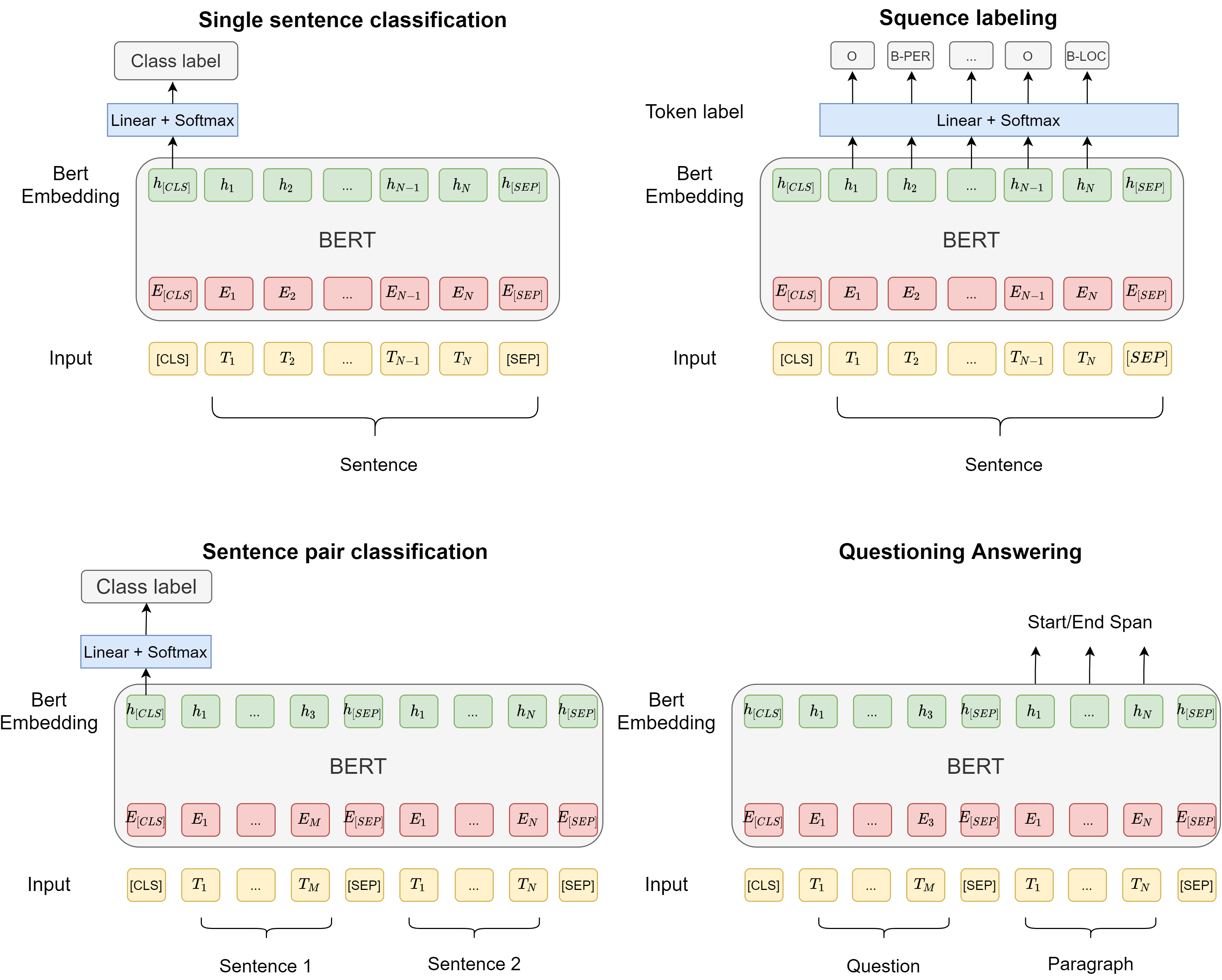
Fig. 6.8 BERT architecture configuration for different downstream tasks.

6.3. Efficient BERT Models

6.3.1. Introduction

BERT has achieved marked success in tackling challenging NLP tasks such as natural language inference, machine reading comprehension, and question answering. In an end-to-end system, BERT can used as an encoder, which connects back-end task-specific modules (e.g., classifiers). By fine-tuning the BERT, the system can usually achieve satisfactory results even under limited resources setting (e.g., small training set). However, BERT is huge model, the base version has 108M parameters, which prohibits its application in devices with limited memory and computation power.

In this section, we are going to review different strategies to develop smaller versions of BERT without significant compromise on its performance.

6.3.2. ALBERT

ALBERT [LCG+20], standing for A Lite BERT, is one of the recent achievement that reduces the model parameter number considerably and at the same time improves performance. In ALBERT , there are three major improvements on the model architecture and the pretraining process. The first two improvements on the model architecture are

• Factorized embedding parameterization. In the original BERT, tokens (represented as one-hot vectors) are directly projected the hidden space with dimensionality \(H = 768\) or \(1024\). For large vocabulary size \(V\) at the scale of 10,000, the projection matrix \(W\) has parameters \(HV\). One way to reduce parameter size is to factorize \(W\) into two lower rank matrices. This is equivalent to two-step projection:

  • First project one-hot vector to embedding space of dimensionality \(E\), say \(E= 128\);

  • Second project the embedding space to the hidden space of dimensionality \(H\). The two-step projection only requires parameters \(VE + EH\) and the reduction is notable when \(E \ll H\).

• Cross-layer parameter sharing. In the original BERT, each encoder sub-unit (which has an attention module and a feed-forward module) has different parameters. In ALBERT, these parameters are shared in different sub-units to reduce model size and improve parameter efficiency. The authors also mentioned that there are alternative parameter sharing strategies: only sharing feed-forward network parameters; only sharing attention module parameters; sharing both feed-forward network and attention module.

The effect of embedding factorization and parameter sharing can be illustrated in the following comparison.

Table 6.2 BERT model parameters

Model	Parameters	Layers	Hidden	Embedding	Parameter-sharing
base	108 M	12	768	768	False
large	334 M	24	1024	1024	False

The third improvement in ALBERT over BERT is a new sentence-level loss to replace the next sentence prediction task. In the original BERT, the next-sentence prediction (NSP)

In ALBERT, a new sentence-order prediction (SOP) loss to model inter-sentence coherence, which demonstrated better performance in multi-sentence encoding tasks was motivated to improve performance on downstream tasks involving reasoning about the relationship between sentence pairs such as natural language inference. However, several follow-up studies [LOG+19] found that the NSP task has minimal impact and was even eliminated in several BERT variants. One possible reason is that there is a lack of difficulty in the NSP task. Specifically, the sentence pair in a negative example are randomly sampled from the corpus, and there could exist a vast topical difference that makes the prediction task much easier than the intended coherence prediction.

In ALBERT, a sentence-order prediction (SOP) loss replaces NSP loss. The SOP loss avoids topic prediction and instead focuses on modeling inter-sentence coherence. The positive example consists of two consecutive segments from the same document; the negative example consists of the same two consecutive segments but with their order swapped. This forces the model to learn a fine-grained representation about sentence level coherence properties.

6.4. Model Distillation

6.4.1. DistillBERT

Knowledge distillation is a knowledge transfer approach to transfer knowledge to a large BERT model (also called a teacher model), to a smaller, ready-to-deploy BERT model (also called a student model) such that the small model can have performance close to the teacher model.

DistilBERT [SDCW19] applies a knowledge distillation method based on triple loss (TripleLoss). Next, the knowledge distillation method used by DistilBERT is introduced.

The DistilBERT model has six Transformer layers, which is the half the total number of BERT \(_{\text {BASE }}\). DistillBERT also removes the token embedding in the input. Compared with the BERT model, the parameters of DistilBERT are compressed to 40% of the original, and at the same time, the reasoning speed is improved, and it reaches 97% of the effect of the BERT model on multiple downstream tasks. The teacher model directly uses the original BERT-base model. The student model uses the first six layers of the teacher model for initialization.

To transfer the knowledge from a teacher model to a student model, DistillBERT employs three types of losses: MLM loss, distillation MLM loss, and cosine similarity loss. Next sentence prediction pretraining task is removed.

The MLM loss is the same as the original BERT model training. The distillation MLM loss is based on the Soft label produced from the teacher model, given by

\[\mathcal{L}_{d-mlm} = - \sum_{i} t_i \log (s_i),\]

where \(t_i\) is the probability on class label \(i\) from the teacher model and \(s_i\) is the probability on the same class from the student model. Note that when we compute the probabilities, we use a temperature parameter \(\tau\) to control the softness of the distribution. For example,

\[t_i = \frac{\exp(z_i^T/\tau)}{\sum_{j}\exp(z_j^T/\tau)},\]

where \(z_i\) is the un-normalized teacher model output.

The Cosine similarity loss is used to align the the directions between the teacher model’s embeddings and the student model’s embeddings, which is given by

\[\mathcal{L}_{cos} = 1 - \operatorname{CosSimilarity}(h^t, s^t)\]

where \(h^t\) and \(s^t\) are last hidden layer outputs from the teacher model and the student model for the same input example, respectively.

6.4.2. TinyBERT

TinyBERT [JYS+19] proposes a novel layer-wise knowledge transfer strategy to transfer more fine-grained knowledge, including hidden states and self-attention distributions of Transformer networks, from the teacher to the student. To perform layer-to-layer distillation, TinyBERT specifies a mapping between the teacher and student layers, and uses a parameter matrix to linearly transform student hidden states.

Assuming that the student model has \(M\) Transformer layers and teacher model has \(N\) Transformer layers. As we need to choose \(M\) out of \(N\) layers from the teacher model for layerwise knowledge transfer distillation, we choose a mapping function \(n=g(m)\) to specify the correspondence between indices from student layers to teacher layers. We consider knowledge transfer in three different layer types: embedding layer, transformer layer, and prediction layer.

Embedding-layer Distillation. Embedding-layer knowledge transfer is realized by matching embedding matrix via a linear transformation. Specifically, we can impose a training objective given by:

\[ \mathcal{L}_{\mathrm{embd}}=\operatorname{MSE}\left(\boldsymbol{E}^{S} \boldsymbol{W}_{e}, \boldsymbol{E}^{T}\right) \]

where the matrices \(\boldsymbol{E}^{S}\) and \(\boldsymbol{H}^{T}\) refer to the embeddings of student and teacher networks, respectively. The matrix \(\boldsymbol{W}_{e}\) is a learnable linear transformation.

Transformer-layer Distillation. The Transformer-layer knowledge distillation includes the self-attention based distillation and hidden-state distillation.

The attention based distillation can transfer rich semantic and syntax knowledge captured in self-attention modules [CKLM19]. Specifically, we impose a training loss to match self-attention matrices between the teacher and the student network, given by:

\[ \mathcal{L}_{\text {attn }}=\frac{1}{H} \sum_{i=1}^{H} \operatorname{MSE}\left(\boldsymbol{A}_{i}^{S}, \boldsymbol{A}_{i}^{T}\right), \]

where \(H\) is the number of attention heads, \(\boldsymbol{A}_{i} \in\) is the attention matrix in the \(i\)-th head of model. It is found that using the unnormalized attention matrix \(\boldsymbol{A}_{i}\) led to a faster convergence rate and better performances.

Compared to the attention based distillation, hidden-state distillation impose matching condition on outputs of Transformer layers via a training loss given by:

\[ \mathcal{L}_{\text {hidn }}=\operatorname{MSE}\left(\boldsymbol{H}^{S} \boldsymbol{W}_{h}, \boldsymbol{H}^{T}\right) \]

where the matrices \(\boldsymbol{H}^{S}\) and \(\boldsymbol{H}^{T}\) refer to the hidden states of student and teacher networks after the feed-forward network. The matrix \(\boldsymbol{W}_{h}\) is a learnable linear transformation to match the dimensionality between the student’s hidden state and the teacher’s hidden states.

Prediction-layer Distillation. The final prediction-layer distillation follows the soft target classification task as in [HVD15]. Specifically, we impose a soft cross-entropy loss between the student network’s logits against the teacher’s logits:

\[ \mathcal{L}_{\text {pred }}=\operatorname{CrossEntropy}\left(\boldsymbol{z}^{T} / \tau, \boldsymbol{z}^{S} / \tau\right) \]

where \(\boldsymbol{z}^{S}\) and \(\boldsymbol{z}^{T}\) are the logits vectors predicted by the student and teacher respectively. \(\tau\) is the temperature.

For simplicity,

Finally, we set 0 to be the index of embedding layer and \(M+1\) to be the index of prediction layer, and the corresponding layer mappings are defined as \(0=g(0)\) and \(N+1=g(M+1)\) respectively. Using the above distillation objectives, we can unify the distillation loss of the corresponding layers between the teacher and the student network:

\[\begin{split} \mathcal{L}_{\text {layer }}= \begin{cases}\mathcal{L}_{\text {embd }}, & m=0 \\ \mathcal{L}_{\text {hidn }}+\mathcal{L}_{\text {attn }}, & M \geq m>0 \\ \mathcal{L}_{\text {pred }}, & m=M+1\end{cases}. \end{split}\]

6.4.3. MobileBERT

MobileBERT [SYS+20] is designed to be as deep as BERT \(_{\text {LARGE }}\) and make each layer much narrower. A deep and narrow Transformer networks have the strength of large modeling capacity like deep network and maintain a manageable model size. To maintain a good balance between self-attentions and feed-forward networks a bottleneck structures is adopted, which amounts to adding projection layers (with activation) before the entry and after the output of each Transformer layer. Direct distill knowledge from \(\mathrm{BERT}_{\text {LARGE }}\) to MobileBERT is challenge due to large discrepancy in the architecture. One solution is to first train a specially designed teacher model, an inverted-bottleneck incorporated \(\mathrm{BERT}_{\text {LARGE }}\) model (IB-BERT). Then, we conduct knowledge transfer from IB-BERT to MobileBERT.

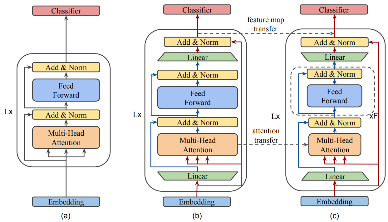
Fig. 6.9 Illustration of three model architectures for model distillation from BERT to MobileBERT.: (a) BERT; (b) Inverted-Bottleneck BERT (IB-BERT); and (c) MobileBERT. We first train IB-BERT and then distill knowledge from IB-BERT to MobileBERT via layerwise knowledge transfer focused on feature map transfer and attention transfer. Image from [SYS+20].

Model distillation from IB-BERT to the student model relies on two layer-wise knowledge transfer training objectives: feature map transfer and attention transfer.

Feature Map Transfer (FMT): BERT layers perform multi-head self-attention as well as nonlinear feature transform via feed-forward layers. The layer-wise knowledge transfer can be facilitated by requiring the feature maps of each layer to be as close as possible to those of the teacher. Here feature map is defined as the output of the FFN layer at each position. In particular, the mean squared error between the feature maps of the MobileBERT student and the IB-BERT teacher is used as the knowledge transfer objective:

\[ \mathcal{L}_{F M T}^{\ell}=\frac{1}{T N} \sum_{t=1}^{T} \sum_{n=1}^{N}\left(H_{t, \ell, n}^{t r}-H_{t, \ell, n}^{s t}\right)^{2}, \]

where \(\ell\) is the index of layers, \(T\) is the sequence length, and \(N\) is the feature map size.

Attention Transfer (AT): The attention mechanism plays a crucial role in the modeling capacity of Transformer and BERT. By requiring the similarity between self-attention maps can also help the training of MobileBERT in augmentation to the feature map transfer. In particular, we minimize the KL-divergence between the per-head self-attention distributions of the MobileBERT student and the IB-BERT teacher:

\[ \mathcal{L}_{A T}^{\ell}=\frac{1}{T A} \sum_{t=1}^{T} \sum_{a=1}^{A} D_{K L}\left(a_{t, \ell, a}^{t r} \| a_{t, \ell, a}^{s t}\right) \]

where \(A\) is the number of attention heads.

The above two layerwise knowledge transfer loss serves as regularization when we pre-train the MobileBERT. We use a linear combination of the original masked language modeling (MLM) loss, next sentence prediction (NSP) loss, and the new MLM Knowledge Distillation (KD) loss as our total loss, given by:

\[ \mathcal{L}=\alpha \mathcal{L}_{MLM} + \mathcal{L}_{NSP} +(1-\alpha) {\mathcal{L}}_{K D} \]

where \(\alpha\) is a hyperparameter in \((0,1)\) and $\(\mathcal{L}_{KD} = \sum_{\ell=1}^L \mathcal{L}^\ell_{FMT} + \mathcal{L}^\ell_{AT}.\)$

Additional model compression strategy includes embedding factorization. The embedding layer in BERT models accounts for a significant portion of model size. MobileBERT adopts raw token embedding dimension to be 128 and apply a 1D convolution with kernel size 3 on the raw token embedding to produce a 512 dimensional output.

6.4.4. MiniLM

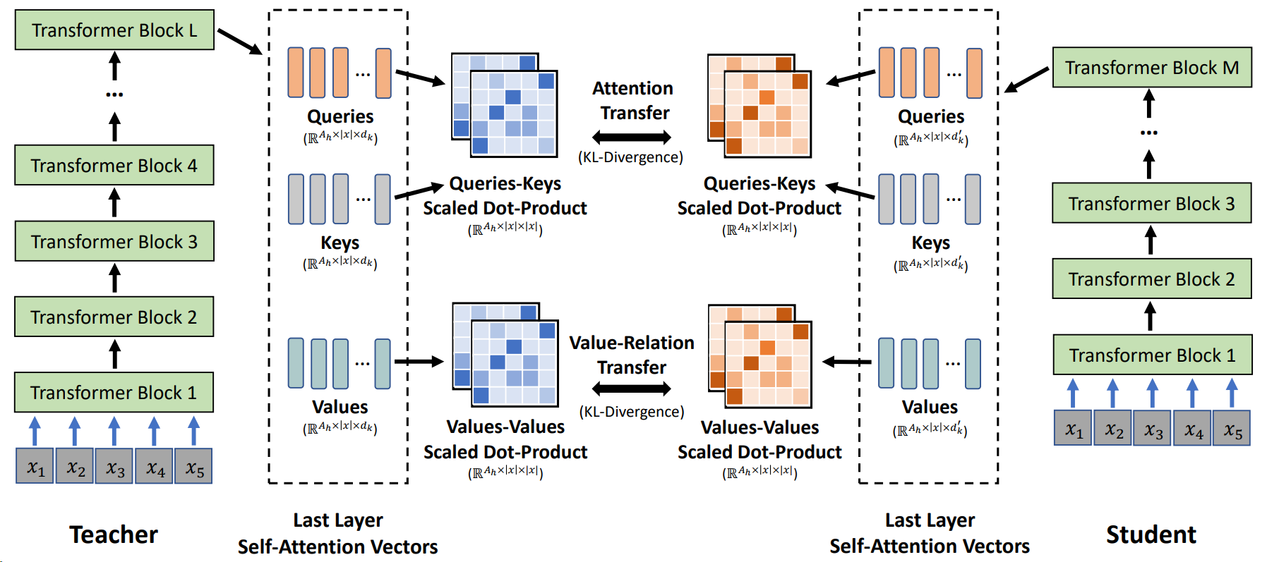
Fig. 6.10 Overview of self-attention knowledge transfer in MiniLM. The student is trained by mimicking the self-attention behavior of the last Transformer layer of the teacher. Two loss functions are used to enable the self-attention distribution transfer and the self-attention value-relation transfer. Image from [WWD+20].

MiniLM [WWD+20] follows similar line of thought like TinyBERT and MobileBERT and focuses on deep mimicking the self-attention modules, which are the fundamentally important components in the Transformer based models.

Specifically, MiniLM proposes only distilling the self-attention module of the last Transformer layer alone of the teacher model, rather than performing layer-to-layer knowledge distillation. Performing layer-to-layer knowledge distillation imposes more requirements on the structure similarity between the teacher and the student and finding proper layer mappings, while nonperforming last layer knowledge distillation allows the choice of the student model architecture to be more flexible.

Compared to self-attention transfer in TinyBERT and MobileBERT, MiniLM performs both Self-Attention Distribution Transfer and Self-Attention Value-Relation Transfer to promote the matching between teacher model and student model in the self-attention module. The additional inner product type of matching is a flexible objective as it does not require the hidden dimensionality between student model and the teach model to be equal.

In the self-attention distributions transfer, one can minimize the KL-divergence between the self-attention distributions, given by

\[ \mathcal{L}_{\mathrm{AT}}=\frac{1}{A_{h}|x|} \sum_{a=1}^{A_{h}} \sum_{t=1}^{|x|} D_{K L}\left(\mathbf{A}_{L, a, t}^{T} \| \mathbf{A}_{M, a, t}^{S}\right) \]

where \(|x|\) and \(A_{h}\) are the sequence length and the number of attention heads. \(L\) and \(M\) denote the number of layers for the teacher and student. \(\mathbf{A}_{L}^{T}\) and \(\mathbf{A}_{M}^{S}\) are the attention distributions of the last Transformer layer in the teacher and student, respectively, which are computed by the scaled dot-product of queries and keys.

The value relation transfer has two steps: first, value relation is computed via the multi-head scaled dot-product between values; second, the KL-divergence between the value relation of the teacher and student is used as the training objective, which is given by $\(\mathcal{L}_{\mathrm{VR}}=\frac{1}{A_{h}|x|} \sum_{a=1}^{A_{h}} \sum_{t=1}^{|x|} D_{K L}\left(\mathbf{V R}_{L, a, t}^{T} \| \mathbf{V R}_{M, a, t}^{S}\right)\)$ where

\[\begin{split} \begin{align} \mathbf{V R}_{L, a}^{T}=\operatorname{Softmax}\left(\frac{\mathbf{V}_{L, a}^{T} \mathbf{V}_{L, a}^{T \top}}{\sqrt{d_{k}}}\right) \\ \mathbf{V R}_{M, a}^{S}=\operatorname{Softmax}\left(\frac{\mathbf{V}_{M, a}^{S} \mathbf{V}_{M, a}^{S_{\top}}}{\sqrt{d_{k}^{T}}}\right) \end{align} \end{split}\]

where \(\mathbf{V}_{L, a}^{T} \in \mathbb{R}^{|x| \times d_{k}}\) and \(\mathbf{V}_{M, a}^{S} \in \mathbb{R}^{|x| \times d_{k}^{\prime}}\) are the values of an attention head in self-attention module for the teacher’s and student’s last Transformer layer. VR \(\mathbf{R}_{L}^{T} \in \mathbb{R}^{A_{h} \times|x| \times|x|}\) and \(\mathbf{V R} \mathbf{R}_{M}^{S} \in \mathbb{R}^{A_{h} \times|x| \times|x|}\) are the value relation of the last Transformer layer for teacher and student, respectively.

Taken together, the distillation loss is the summation between the attention distribution transfer loss and value-relation transfer loss:

\[ \mathcal{L}=\mathcal{L}_{\mathrm{AT}}+\mathcal{L}_{\mathrm{VR}}. \]

6.4.5. Sample Efficient: ELECTRA

ELECTRA (Efficiently Learning an Encoder that Classifies Token Replacements Accurately) [CLLM20] is proposed to improve the BERT pretraining efficiency when there is a pretraining computation budget.

The key innovation in ELECTRA is the proposition of a new generator-discriminator training framework. This framework shares some similarity to but not equivalent to adversarial training (e.g., GAN). As shown in Fig. 6.11, The generator \(G\), typically a masked language model, produces an output distribution over masked tokens for replacement purpose. The generator is trained to predict masked tokens and the discriminator \(D\) is trained to distinguish which token is replaced. In contrast to GAN, the gradient of discrimination loss will not passed down to the generator to train the generator to generate adversarial examples. In addition, no NSP pre-training task is performed.

The major benefits arising from novel architectures are two folds.

• The classical masked language modeling (MLM) approaches is not sample efficient since the network only learns from \(15 \%\) of the tokens per example. On the other hand, ELECTRA performs discrimination task on all tokens rather than generative task on just masked tokens.

• This token replacement procedure reduces the mismatch phenomenon during fine-tuning for BERT models. That is, there is are mask tokens in the input sequence during fine-tuning but there is no mask tokens during inference.

Both generator \(G\) and discriminator \(D\) can use the transformer encoder architecture. The encoder maps a sequence on input tokens \(x=\) \(\left[x_{1}, \ldots, x_{n}\right]\) into a sequence of contextualized vector representations \(h(\boldsymbol{x})=\left[h_{1}, \ldots, h_{n}\right]\). For a masked token \(x_{t}\), the generator outputs a probability distribution via:

\[ p_{G}\left(x_{t} \mid \boldsymbol{x}\right)=\exp \left(e\left(x_{t}\right)^{T} h_{G}(\boldsymbol{x})_{t}\right) / \sum_{x^{\prime}} \exp \left(e\left(x^{\prime}\right)^{T} h_{G}(\boldsymbol{x})_{t}\right) \]

where \(e\) denotes token embeddings. The replaced token is then sampled from this distribution.

Given an input sequence with sampled replaced token, the discriminator predicts whether each token \(x_{t}\) is replaced or is original via:

\[ D(\boldsymbol{x}, t)=\operatorname{sigmoid}\left(w^{T} h_{D}(\boldsymbol{x})_{t}\right) \]

The loss function for the generator is the same as masked language modeling loss, given by

\[ \mathcal{L}_{\mathrm{MLM}}\left(\boldsymbol{x}, \theta_{G}\right)=\mathbb{E}\left(\sum_{i \in masked}-\log p_{G}\left(x_{i} \mid \boldsymbol{x}^{\text {masked }}\right)\right). \]

The loss function for the discriminator is

\[\mathcal{L}_{Disc}\left(\boldsymbol{x}, \theta_{D}\right)=\mathbb{E}\left(\sum_{t=1}^{n}-y_t \log D\left(\boldsymbol{x}^{\text {replaced }}, t\right)-\left(1 - y_t\right) \log \left(1-D\left(\boldsymbol{x}^{\text {replaced }}, t\right)\right)\right).\]

where \(y_t\) is a binary label with 1 indicating \(x_t\) is a replaced token and 0 otherwise. As the generator is trained, the replaced tokens is harder and harder to distinguish, which further improves the learning of the discriminator.

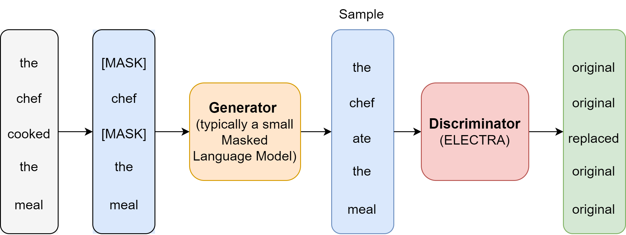
Fig. 6.11 Illustration of the generator-discriminator training framework. The generator, typically a masked language model, produces an output distribution over masked tokens for replacement purpose. The generator encoder is trained to predict masked tokens and the discriminator is trained to distinguish which token is replaced. After pre-training, the generator is discarded and only the discriminator encoder is fine-tuned on downstream tasks.

The authors show that when is the compute budget on pretraining, ELECTRA can significantly outperform BERT. Ablation studies show that the major gain is coming from sample efficiency and the minor gain is coming from mismatch reduction.

6.5. Multilingual Models

6.5.1. Introduction

In this section, we discuss the possibility of obtaining a universal representation for different languages [AST18]. In other words, when we pretrain a language model on corpus in different languages, the pretrained encoder is able to represent different language symbols and tokens in the same semantic vector space. This unified representation can benefit cross-lingual language processing tasks, such as translation.

One application of cross-lingual ability is to fine-tune a pretrained multilingual language model on one language for a specific task, and the model automatically acquire the capability to perform the same task in another target language (which is also known as Zero-shot transfer). This application is attractive when we don’t have enough training data in the target language, for example, low-resource languages. Another application scenario is to fine-tuning model in multiple languages at the same time; such cross-lingual training can improve the overall performance on all of these languages. In [GarciaJSValdes17], it is shown that a single shared sequence-to-sequence LSTM encoder-decoder model can be used to perform machine translation for multiple language pairs.

For independently learned static word embeddings (e.g., word2vec) in different languages, the embeddings corresponding to similar semantics are usually vastly different. To encode tokens of different languages into the same semantic space, one can align (i.e., translate and rotate) two different semantic vectors space by requiring tokens and their translated tokens have similar embeddings in the same semantic vector. The alignment or conversion can be realized via translation matrix, which maps one’s language embedding vector into another language’s embedding space.

On the other hand, for independently learned contextualized word embedding (e.g., BERT) in different language, there is no straight forward approach like translation matrix to make this conversion. Instead, one require pretraining a language model on multilingual corpus with parallel sentence pairs (i.e., sentences pairs in different languages but with similar meanings).

In the section, we will go over different approaches to obtaining cross-lingual ability from pretrained language models.

6.5.2. Multilingual-BERT (mBERT)

When Google published their pretrained BERT model in English, they also published a multilingual-BERT which is trained on the wikipedia in the most popular 104 languages. Although the model is trained on corpus without explicitly aligned parallel sentence, mBERT surprisingly acquire some level of cross-lingual representation and understanding abilities.

The multilingual BERT model adopts the same pre-training task (i.e., masked language modeling and next sentence prediction) and model structure as the monolingual BERT, and all languages are encoded and represented by the same architecture except that the tokenizer is trained on multi-lingual setting and has a vocabulary size 110k.

Why simply pre-training on multilingual mixed data can help the model acquire cross-lingual ability and represent the tokens of different language in the same semantic space? This is mainly because the training corpus itself has mixed use and shared subwords across languages. The so-called mixed use, that is, texts in one language are often mixed with other languages, is quite common for languages that have the same origin and share some subset of their vocabularies. Even in languages with vastly different origins, there are mixed usages, either intentionally or unintentionally.

For example, some scientific article in Chinese might also contains a large number of English terms. The tokenization strategy used by BERT further increases the size of the shared vocabulary as the root of some words from different languages is the same.

These shared vocabulary or subwords ultimately serve as connections between different languages and enables multiple languages to be represented in the same semantic space. However, if too few words are shared between languages, this can cause problems for this type of training approach.

Although there is no need to use bilingual parallel sentence pairs, and only the data of each language needs to be sampled separately. Because the imbalance training samples from different languages, specific sampling strategy is needed to improve the performance for small languages.

6.5.3. XLM, XLM-R, And XLM-E

One source where mBERT acquires its cross-lingual ability is from the shared vocabulary and subwords cross languages. However, for some languages, the training might suffer from the lack of shared vocabulary in monolingual dominant corpora (e.g., wikipidia). XLM (Cross-lingual Language Model Pretraining) [LC19] adapted BERT’s unsupervised pre-training masked language modeling to multi-lingual settings and proposed an additional supervised learning strategy known as Translation Language Modeling (TLM) [Fig. 6.12].

Compared to BERT’s masked language modeling, multilingual masked language modeling (MMLM) uses text streams of an arbitrary number of sentences (truncated at 256 tokens) instead of pairs of sentences. To offset the imbalance between rare and frequent tokens (e.g. punctuations or stop words), the probability of a token being masked is adjusted to be proportional to the square root of their invert frequencies.

TLM is based on predicting masked words on parallel sentence pairs (i.e., sentences that are translated to each other). The idea is that when one language provides insufficient information for prediction, the translation in another language can provide additional supplementary information. Specifically, words in both the source and target sentences are randomly masked. To predict a word masked in an English sentence, the model is allowed to attend both surrounding English words as well as to its French translation. To facilitate the alignment, the positions of target sentences are reset.

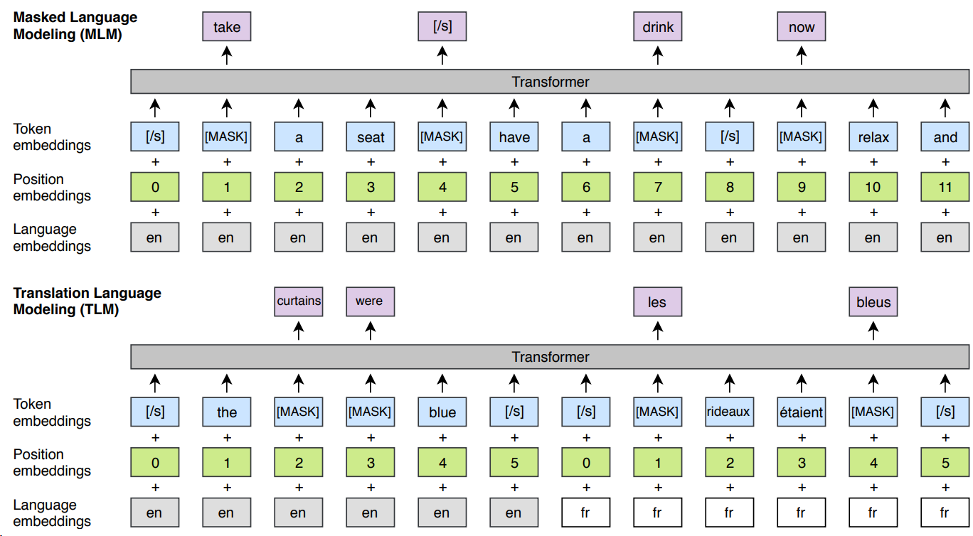
Fig. 6.12 Cross-lingual language model pretraining has a unsupervised multi-lingual masked language modeling (MMLM) task (top) as well as a supervised translational language modeling (TLM) task (bottom). The TLM objective extends MMLM to pairs of parallel translated sentences. To predict a masked English word, the model can attend to both the English sentence and its French translation. Position embeddings of the target sentence are reset to facilitate the alignment. Image from [LC19].

Although XLM achieves better results than mBERT, it relies on bilingual parallel sentence pairs. However, it is difficult to obtain large-scale sentence pair data in many languages. In addition, bilingual parallel data is generally sentence-level, which makes it impossible to use a wider range of contextual information beyond sentences, thus causing a certain loss to the performance of the model. In order to solve this problem, Facebook has improved XLM and proposed the XLM-R (XLM-RoBERTa) model[CKG+19]. As the name suggests, the model structure of XLM-R is consistent with RoBERTa, and the biggest difference from XLM is that the pre-training task of the translation language model is removed, so that it no longer relies on bilingual parallel corpora. In order to further improve the effect of the model on small languages, XLM-R also uses the larger CommonCrawl multilingual corpus. In order to improve the cross-lingual ability of the pretrained model, one can also manually perform code-switch to enrich the training data.

To make XLM more sample efficient in the pretraining process, we can adopt ELECTRA style discriminator training in the multi-lingual setting. In XLM-E[CHD+21], two discriminative pre-training tasks, namely multilingual replaced token detection, and translation replaced token detection, are introduced. As shown in Sample Efficient: ELECTRA, the two tasks build input sequences by replacing tokens in multilingual sentences and translation pairs. The multilingual replaced token detection task requires the model to distinguish real input tokens from corrupted monolingual sentences in different languages. Both the generator and the discriminator are shared across languages. The vocabulary is also shared for different languages. The task is the same as in monolingual ELECTRA pre-training.

In the Translation Replaced Token Detection task, we have parallel translated sentences as the input. The detection of replaced tokens is allowed to attend to surrounding words in the same language and words in the translated input.

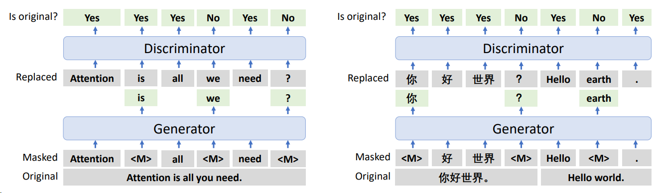
Fig. 6.13 The multilingual replaced token detection and translation replaced token detection pretraining tasks for XLM-E pre-training. The generator predicts the masked tokens given a masked sentence or a masked translation pair, and the discriminator distinguishes whether the tokens are replaced by the generator. Image from [CHD+21].

6.5.4. The EXTREME Benchmark

One of the most common benchmark test for cross-lingual transferability is the XTREME benchmark [HRS+20], which stands for Cross-lingual TRansfer Evaluation of Multilingual Encoders. This benchmark covers 40 typologically diverse languages that span 12 language families, and it includes 9 tasks that require reasoning on different levels of syntax or semantics.

The tasks included in XTREME includes sentence text classification, structured prediction, sentence retrieval and cross-lingual question answering. Consequently, for models to be successful on the XTREME benchmarks, they must learn representations that generalize to many standard cross-lingual transfer settings.

One example sentence text classification task is the Cross-lingual Natural Language Inference, where crowd-sourced English data is translated to ten other languages by professional translators and used for evaluation. The cross-lingual model needs to determine whether a premise sentence entails, contradicts, or is neutral toward a hypothesis sentence.

In the structured prediction task, the model is evaluated on POS tagging task. The model is trained on the English data and then is evaluated on the test sets of the target languages.

6.6. Bibliography

[AST18]

Armen Aghajanyan, Xia Song, and Saurabh Tiwary. Towards language agnostic universal representations. arXiv preprint arXiv:1809.08510, 2018.

[CHD+21] (1,2)

Zewen Chi, Shaohan Huang, Li Dong, Shuming Ma, Saksham Singhal, Payal Bajaj, Xia Song, and Furu Wei. Xlm-e: cross-lingual language model pre-training via electra. arXiv preprint arXiv:2106.16138, 2021.

[CKLM19]

Kevin Clark, Urvashi Khandelwal, Omer Levy, and Christopher D Manning. What does bert look at? an analysis of bert's attention. arXiv preprint arXiv:1906.04341, 2019.

[CLLM20]

Kevin Clark, Minh-Thang Luong, Quoc V Le, and Christopher D Manning. Electra: pre-training text encoders as discriminators rather than generators. arXiv preprint arXiv:2003.10555, 2020.

[CKG+19]

Alexis Conneau, Kartikay Khandelwal, Naman Goyal, Vishrav Chaudhary, Guillaume Wenzek, Francisco Guzmán, Edouard Grave, Myle Ott, Luke Zettlemoyer, and Veselin Stoyanov. Unsupervised cross-lingual representation learning at scale. arXiv preprint arXiv:1911.02116, 2019.

[DCLT18] (1,2,3)

Jacob Devlin, Ming-Wei Chang, Kenton Lee, and Kristina Toutanova. Bert: pre-training of deep bidirectional transformers for language understanding. arXiv preprint arXiv:1810.04805, 2018.

[GarciaJSValdes17]

Ofelia García, Susana Ibarra Johnson, Kate Seltzer, and Guadalupe Valdés. The translanguaging classroom: Leveraging student bilingualism for learning. Caslon Philadelphia, PA, 2017.

[HVD15]

Geoffrey Hinton, Oriol Vinyals, and Jeff Dean. Distilling the knowledge in a neural network. arXiv preprint arXiv:1503.02531, 2015.

[HRS+20]

Junjie Hu, Sebastian Ruder, Aditya Siddhant, Graham Neubig, Orhan Firat, and Melvin Johnson. Xtreme: a massively multilingual multi-task benchmark for evaluating cross-lingual generalisation. In International Conference on Machine Learning, 4411–4421. PMLR, 2020.

[JYS+19]

Xiaoqi Jiao, Yichun Yin, Lifeng Shang, Xin Jiang, Xiao Chen, Linlin Li, Fang Wang, and Qun Liu. Tinybert: distilling bert for natural language understanding. arXiv preprint arXiv:1909.10351, 2019.

[LC19] (1,2)

Guillaume Lample and Alexis Conneau. Cross-lingual language model pretraining. arXiv preprint arXiv:1901.07291, 2019.

[LCG+20]

Zhenzhong Lan, Mingda Chen, Sebastian Goodman, Kevin Gimpel, Piyush Sharma, and Radu Soricut. Albert: a lite bert for self-supervised learning of language representations. 2020. URL: https://arxiv.org/abs/1909.11942, arXiv:1909.11942.

[LKB20]

Qi Liu, Matt J Kusner, and Phil Blunsom. A survey on contextual embeddings. arXiv preprint arXiv:2003.07278, 2020.

[LOG+19] (1,2)

Yinhan Liu, Myle Ott, Naman Goyal, Jingfei Du, Mandar Joshi, Danqi Chen, Omer Levy, Mike Lewis, Luke Zettlemoyer, and Veselin Stoyanov. Roberta: a robustly optimized bert pretraining approach. arXiv preprint arXiv:1907.11692, 2019.

[PNI+18]

Matthew E Peters, Mark Neumann, Mohit Iyyer, Matt Gardner, Christopher Clark, Kenton Lee, and Luke Zettlemoyer. Deep contextualized word representations. arXiv preprint arXiv:1802.05365, 2018.

[QSX+20]

missing journal in Qiu2020PreTrained

[SDCW19]

Victor Sanh, Lysandre Debut, Julien Chaumond, and Thomas Wolf. DistilBERT, a distilled version of BERT: smaller, faster, cheaper and lighter. ArXiv:1910.01108, 2019.

[SYS+20] (1,2)

Zhiqing Sun, Hongkun Yu, Xiaodan Song, Renjie Liu, Yiming Yang, and Denny Zhou. Mobilebert: a compact task-agnostic bert for resource-limited devices. arXiv preprint arXiv:2004.02984, 2020.

[WWD+20] (1,2)

Wenhui Wang, Furu Wei, Li Dong, Hangbo Bao, Nan Yang, and Ming Zhou. Minilm: deep self-attention distillation for task-agnostic compression of pre-trained transformers. Advances in Neural Information Processing Systems, 33:5776–5788, 2020.

[WSC+16]

Yonghui Wu, Mike Schuster, Zhifeng Chen, Quoc V Le, Mohammad Norouzi, Wolfgang Macherey, Maxim Krikun, Yuan Cao, Qin Gao, Klaus Macherey, and others. Google's neural machine translation system: bridging the gap between human and machine translation. arXiv preprint arXiv:1609.08144, 2016.