15. LLM Training Acceleration (WIP)

15.1. The Memory Requirement For Training LLM

We will discuss the following in this section

• How much GPU memory do you need to train \(X\) billion Transformer based LLM per each GPU device.

• What is the formula to estimate memory requirements.

• What would you do in practise to reduce the memory needs if the model does not fit.

15.1.1. Model and Optimizer States

Consider the case that we train a LLM using Adam optimizer, we need to have enough GPU memory to store

• Copy of model parameter

• Copy of model parameter gradients

• Copy of optimizer states, include copy of the model parameters, momentum, and variance.

Assume that

• Model parameters and graidents are stored in FP16 (2 bytes),

• Optimizer states are stored in FP32 (4 bytes) for stable training then training a \(X\) billion model requires following GPU memory amount just to store the model and training states

\[(2 + 2 + 12) X ~\text{(GB)}.\]

The following table gives the example for the memory requirement for models of different sizes.

Model Size	GPU Memory
0.5B	8 GB
3B	48 GB
7B	112 GB
70B	1120 GB

15.1.2. Activations

Let’s have the following notations: \(b\) is the batch size, \(s\) is the sequence length, \(d\) is the model hidden dim, \(L\) is number of layers, \(p\) is the byte size per model paraemters (e.g., 2 for float16). The multiplier 2 is because of both K and V are cached.

Based on the FFN architecture detailed in Pointwise FeedForward Layer, we can estimate the memory requireement for FFN activations

Component	Memory	Note
First Layer	\(4bsdp\)	Output dimension is \(4h\)
Activation	\(4bsdp\)
Second Layer	\(4bsdp\)
Dropout Layer	\(sbd\)
Total	\(9bsdp + bsd\)

Based on the MHA architecture detailed in Multihead Attention with Masks, we can estimate the memory requireement for MHA activations.

Component	Memory	Note
Q/K/V projection	\(3bsdp\)
Softmax input and output	\(2bs^2Hp\)	\(s\times s\) attention matrix for each head
Dropout after Softmax	\(bs^2H\)
Output from \(H\) attention head	\(bsdp\)
Output layer (\(W_O\))	\(bsdp\)
Dropout	\(bsd\)
Total	\(5bsdp + 2bs^2Hp + bsd + bs^2H\)

Additionally, there are two Normalization Layers in each Transformer Layer, the output from each such layer will require in total \(2bsdp\) bytes.

Now we arrive at the total amount of bytes required to store the activations for a \(L\) layer Transformer:

\[M_{\text{per layer}} = \underbrace{17bsdp}_{Linear Layer} + \underbrace{2bs^2Hp}_{Softmax} + \underbrace{2bsd + bs^2H}_{Dropout}\]

If we ignore the small quantity \(2bsd\) and take \(p = 2\) (which is float16, 2bypte), we have

\[M_{approx} = (34bsd + 5bs^2H)\times L\]

The implication on activation memory requirement are

• \(M\) scales linearly with batch size

• \(M\) scales linearly with layer number

• \(M\) scales quadratically with sequence length. During training, we cannot afford large context windows.

• Using technique like GQA [Grouped Query Attention (GQA)] can help save training memory.

Using the model training config from Qwen2 model [YYHBZ24], we have the following summary on the activation GPU memory requirement for setting batch size to 1.

Model Size	\(L\)	\(d\)	\(s\)	\(H\)	\(b\)	GPU Memory
0.5B	24	896	4096	14	1	2.9 GB + 2 GB = 4.9 GB
7B	28	3584	4096	28	1	3.9 GB + 4 GB = 7.9GB
72B	64	8192	4096	64	1	71 GB + 8 GB = 79GB

15.1.3. Activation Checkpointing Techniques

LLM have an enormous number of parameters. In the typical backpropogation during training, we save all the activation values from the forward pass to compute gradient, which consumes a large amount of GPU memory.

On one extreme, we can completely discard the activation values from the forward pass and recalculate the necessary activation values when computing gradients. While this mitigates the activation memory footprint issue, it increases the computational load and slows down training.

Gradient Checkpointing [CXZG16] sits in the middle of these two approaches. This method employs a strategy that selects and saves a portion of the activation values from the computational graph, discarding the rest. The discarded activation values need to be recalculated during gradient computation.

Specifically, during the forward pass, activation values of computational nodes are calculated and saved. After computing the next node, the activation values of intermediate nodes are selectively discarded. During backpropagation, saved activations for gradient computation are used directly. If not, the actitions of the current node are recalculated using the saved activations from the previous node.

15.2. Mixed Precision Training

15.2.1. Overview

Training billion-scale LLM requires huge number of memory, which include model loading, optimizer state storage, and gradient storage. The idea of using low-precision for precision-insensitive computation and high-recision for precision sensitive computation leads to Mixed-precision training[MNA+17]. Mixed-precision training lowers the required resources by using lower-precision arithmetic, and it therefore widely used in LLM training. It has the following benefits.

Reduced memory footprint: Mixed precision training leverages half-precision floating point format (FP16), which uses only 16 bits per number, in contrast to the 32 bits used by single precision (FP32). This significant reduction in memory usage offers two key advantages:

1. Enables training of larger models: With the same memory constraints, developers can design and train models with more parameters or greater complexity.

2. Allows for larger minibatches: Increased batch sizes can lead to more stable gradients and potentially faster convergence in some cases.

Accelerated training and inference: The performance gains from mixed precision training stem from two main factors:

1. Reduced memory bandwidth usage: Since FP16 requires half the memory bandwidth of FP32, layers that are memory-bound can see substantial speed improvements.

2. Faster arithmetic operations: Many modern GPUs have specialized hardware for FP16 (and lower precision like int8, FP8) operations , allowing them to perform these calculations much faster than FP32 operations. These factors combine to potentially shorten both training and inference times, especially for large models or when processing substantial amounts of data.

15.2.2. Training Process

This section describes three techniques for successful training of DNNs with half precision: accumulation of FP16 products into FP32; loss scaling; and an FP32 master copy of weights. With these techniques NVIDIA and Baidu Research were able to match single-precision result accuracy for all networks that were trained.[MNA+17]

As shown in Fig. 15.1, key steps in the mixed-precision training are

• Maintain a master copy of model parameters, optimizer momentums and variances with fp32 precision.

• Before the model forward pass begins, allocate new storage to save model parameters in the fp16 format.

• Perform forward pass, the produced activations will be saved as fp16.

• Perform backward pass, the produced gradients will be saved as fp16.

• Use fp16 gradients to update model parameters that are saved as fp32.

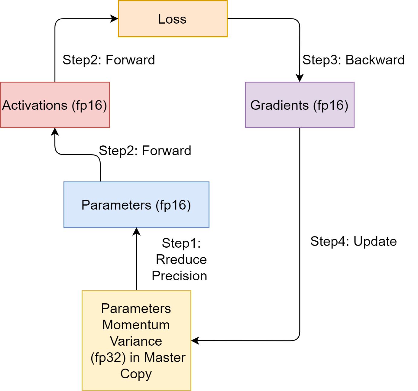
Fig. 15.1 Model training step with mixed precision using classifical Adam algorithm [Algorithm 11.2].

We can estimate the memory storage consumption according to the following table. Denote the model parameter size by \(\Phi\). Let the storage unit be byte. We need \(16\Phi\) memory storage in total.

Table 15.1 Storage requirement for different components during LLM training using Adam.

Type	Storage Size
Parameter (fp32)	\(4 \Phi\)
Momentum(fp32)	\(4 \Phi\)
Variance (fp32)	\(4 \Phi\)
Parameter (fp16)	\(2 \Phi\)
Gradients (fp16)	\(2 \Phi\)
Total:	\(16 \Phi\)

15.3. Distributed Parallel Training

15.3.1. Overview of parallel training techniques

15.3.2. Model parallelism (tensor parallelism)

15.4. ZeRO Via DeepSpeed

Data parallelism is the most widely used technique because it is simple and easy to implement. However, tt is typically challenging to apply the vanilla flavor data parallelism since it requires each GPU to store the parameters of the whole model. As a result, the size of GPU memory becomes the ceiling of the model scale we can train.

Model parallelism (e.g, Megatron) [Model parallelism (tensor parallelism)], desipte its success in T5 (11B) and Megatron-LM (8.3B) is hard to scale beyond model sizes that cannot fit into a single GPU node. This is because model parallelism typically partitions the model weights or layers across GPU devices, incurring a significant communication between devices.

ZeRO (Zero Redundancy Optimizer) [RRRH20] adopt the data parallism paradigm, and optimize memory efficieny and commnication efficiency.

15.4.1. GPU Memory Allocation

GPU memory is mainly allocated into two parts: model states and residual states.

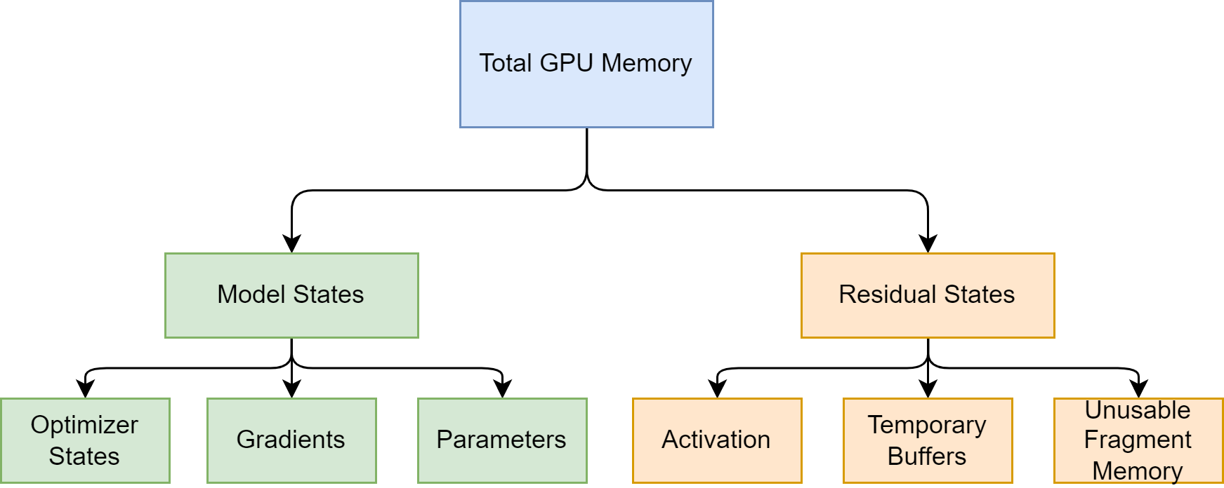
Fig. 15.2 Model training step with mixed precision.

Model states refer to the content that is closely related to the model itself and must be stored. Specifically, they include: \begin{itemize} \item Optimizer states: momentum and variance in the Adam optimization algorithm. \item Gradients: model gradients \item Parameters: model parameters \end{itemize}

Residual States refer to the content that is not necessary for the model, but is generated during the training process. Specifically, they include: \begin{itemize} \item Activation: activation values. We have discussed this in detail in pipeline parallelism. It is used when calculating gradients using the chain rule in the backward process. It can speed up gradient calculation, but it is not necessary to store because it can be calculated by redoing the Forward process. \item Temporary buffers: temporary storage. For example, storage generated when aggregating gradients sent to a GPU for summation. \item Unusable fragment memory: fragmented storage space. Although the total storage space is sufficient, if contiguous storage space cannot be obtained, related requests will also fail. Memory defragmentation can solve this type of space waste. \end{itemize}

15.4.2. ZeRO-Stage-One

Here’s the English translation of the provided text:

(1) \(P_{os}\) (Optimizer State Partitioning) ZeRO-Stage-One reduces the required memory on each device by partitioning the optimizer state across \(N_d\) data-parallel processes. Each process only stores and updates its corresponding partition of the optimizer state, which is \(\frac{1}{N_d}\) of the total optimizer state. At the end of each training step, results from each process are collected to obtain the overall updated state parameters.

(2) The result after ZeRO-Stage1 memory optimization, mainly targeting the optimizer state :

\[ (2+2) \Psi+\frac{K \times \Psi}{N_d} \]

As can be seen, the optimizer state memory has a divisor of \(N_d\) compared to the original.

Example 15.1

For a 7.5B parameter model, the standard case requires 120 GB of memory, but using \(P_{os}\) with \(N_d=64\) only requires 31.4 GB of memory. When \(N_d\) is very large, the memory consumption approaches:

\[ (2+2) \Psi+\frac{K \times \Psi}{N_d} \approx 4 \Psi \]

The ratio compared to the original:

\[ \frac{4}{4+K} \]

When \(K=12\), this becomes \(\frac{1}{4}\), meaning the memory usage is \(\frac{1}{4}\) of the original.

15.5. Appendix

15.5.1. Floating Data Types

Float32 (FP32) stands for the standardized IEEE 32-bit floating point representation. With this data type it is possible to represent a wide range of floating numbers. In FP32, 8 bits are reserved for the “exponent”, 23 bits for the “mantissa” and 1 bit for the sign of the number. In addition to that, most of the hardware supports FP32 operations and instructions.

In the float16 (FP16) data type, 5 bits are reserved for the exponent and 10 bits are reserved for the mantissa. This makes the representable range of FP16 numbers much lower than FP32. This exposes FP16 numbers to the risk of overflowing (trying to represent a number that is very large) and underflowing (representing a number that is very small).

For example, if you do 10k * 10k you end up with 100M which is not possible to represent in FP16, as the largest number possible is 64k. And thus you’d end up with NaN (Not a Number) result and if you have sequential computation like in neural networks, all the prior work is destroyed. Usually, loss scaling is used to overcome this issue, but it doesn’t always work well.

A new format, bfloat16 (BF16), was created to avoid these constraints. In BF16, 8 bits are reserved for the exponent (which is the same as in FP32) and 7 bits are reserved for the fraction.

This means that in BF16 we can retain the same dynamic range as FP32. But we lose 3 bits of precision with respect to FP16. Now there is absolutely no problem with huge numbers, but the precision is worse than FP16 here.

In the Ampere architecture, NVIDIA also introduced TensorFloat-32 (TF32) precision format, combining the dynamic range of BF16 and precision of FP16 to only use 19 bits. It’s currently only used internally during certain operations.

In the machine learning jargon FP32 is called full precision (4 bytes), while BF16 and FP16 are referred to as half-precision (2 bytes). On top of that, the int8 (INT8) data type consists of an 8-bit representation that can store \(2^8\) different values (between [0, 255] or [-128, 127] for signed integers).

While, ideally the training and inference should be done in FP32, it is two times slower than FP16/BF16 and therefore a mixed precision approach is used where the weights are held in FP32 as a precise “main weights” reference, while computation in a forward and backward pass are done for FP16/BF16 to enhance training speed. The FP16/BF16 gradients are then used to update the FP32 main weights.

During training, the main weights are always stored in FP32, but in practice, the half-precision weights often provide similar quality during inference as their FP32 counterpart – a precise reference of the model is only needed when it receives multiple gradient updates. This means we can use the half-precision weights and use half the GPUs to accomplish the same outcome.

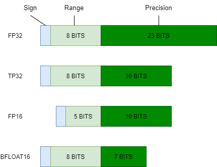
Fig. 15.3 Comparison of different float number types.

15.5.2. GPU Parallel Operations

References https://docs.nvidia.com/deeplearning/nccl/user-guide/docs/usage/collectives.html#:~:text=The ReduceScatter operation performs the same operation as,mapping since the ranks determine the data layout.

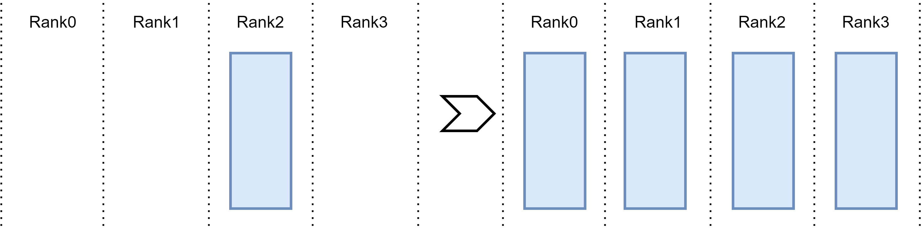
Fig. 15.4 Broadcast operation: data in one device is sent to all other devices.

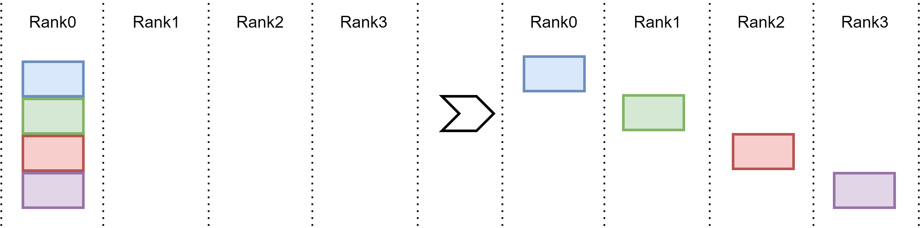
Fig. 15.5 Scatter operation.

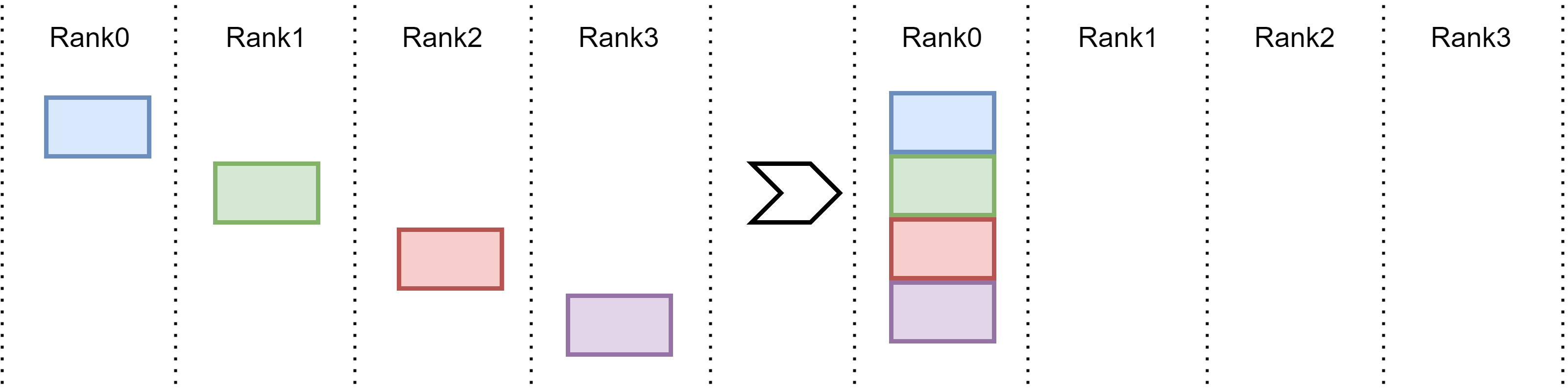
Fig. 15.6 Gather operation: every device broadcasts their data patition to a designated devices. Eventually, this desigated device has the complete data.

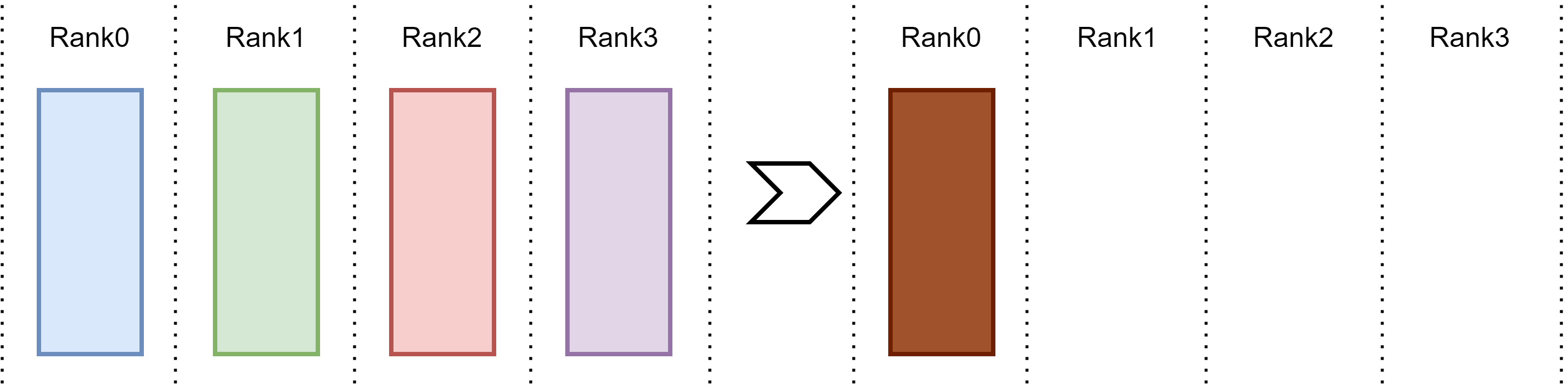
Fig. 15.7 Reduce operation.

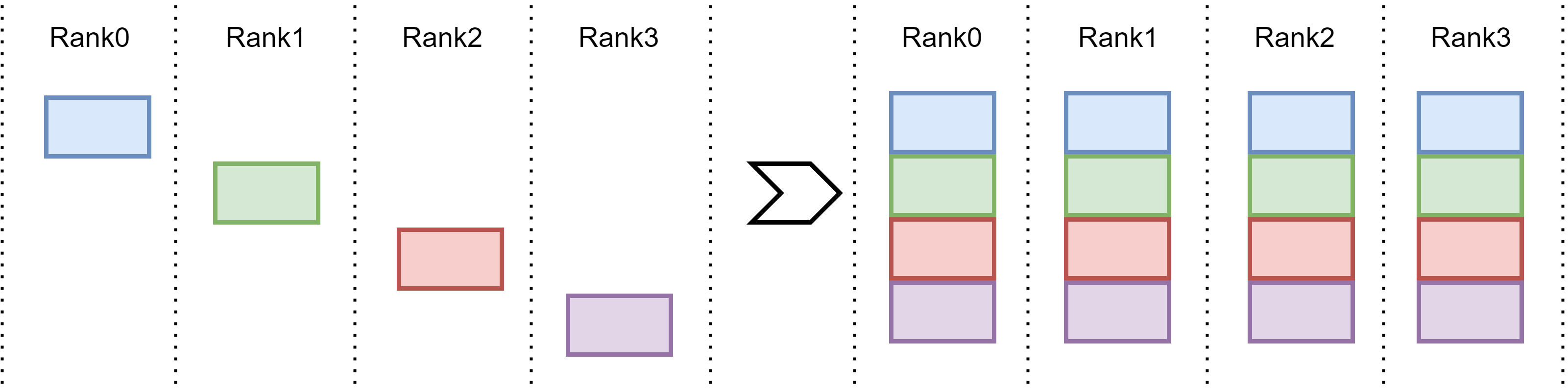
Fig. 15.8 AllGather operation: every device broadcasts their chuck of data to all other devices. Eventually, every device has a complete data copy.

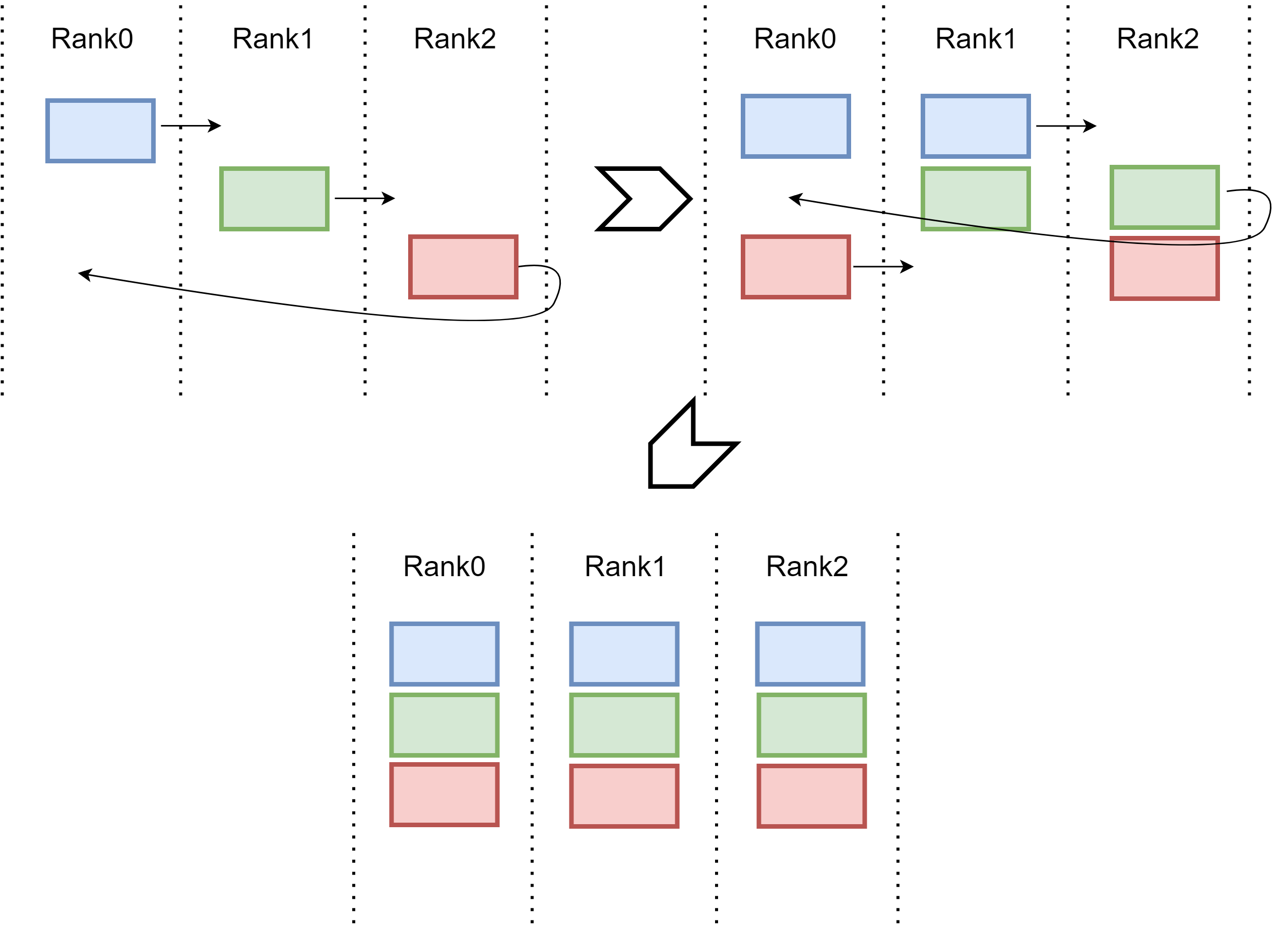
Fig. 15.9 Communication efficient implementation for AllGather via ring style. Every device sends its chuck of data to the next device in the ring.

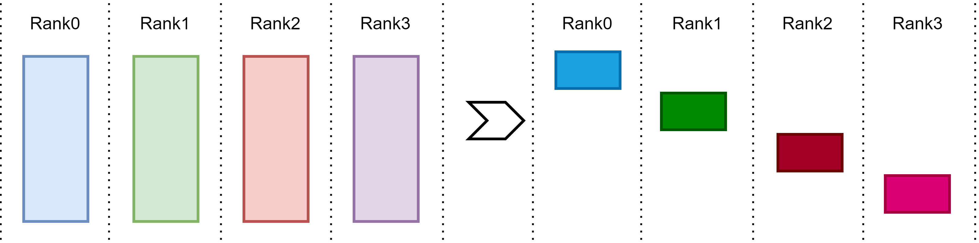
Fig. 15.10 ReduceScatter operation performs the same operation as Reduce, except that the result is scattered in equal-sized blocks across devices.

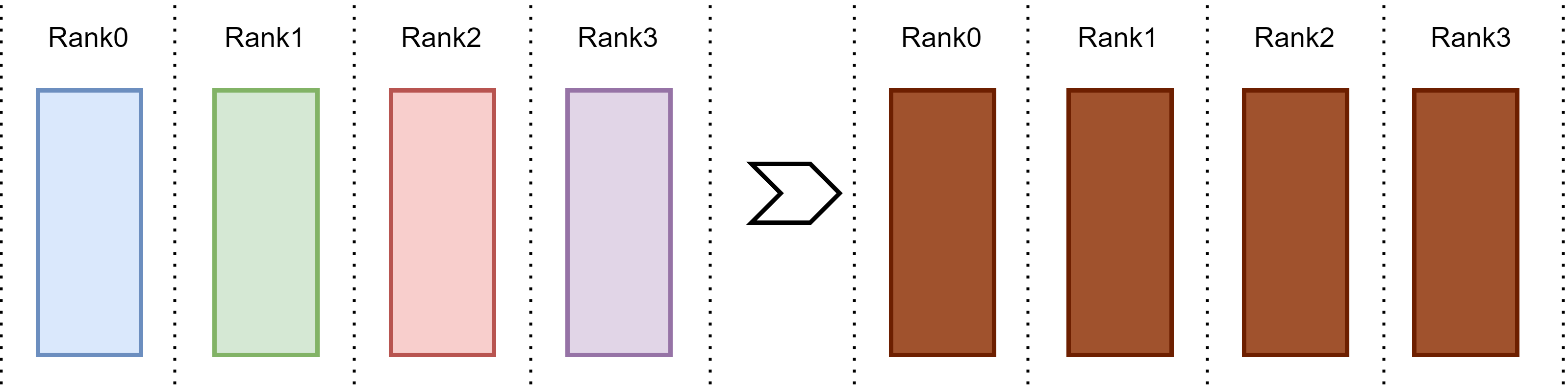
Fig. 15.11 AllReduce operation.

A naive AllReduce implementation would be two steps:

1. Reduce: All devices first send their data to Rank0 device, and performing reduce operation on Rank0.

2. Broadcast: the reduce results are sent to all other devices. This amounts to a total \(2(N_d-1)\Phi\) communication volume, in which the step 1 has \((N_d-1)\Phi\) and step 2 has \((N_d-1)\Phi\). The naive implementation has the communication load imbalance issue as all data are sent into and sent out from Rank0 device.

The RingAllReduce address the load imbalance issue by engaging all devices in data communication and reduction (i.e., more parallelism). The RingAllReduce is equivalent to first RingReduceScatter and then AllGather.

Table 15.2 Communication volumne summary for different operations. Let \(\Phi\) be the total data size in one device and \(N\) be the total number of devices.

Type	Storage Size
Broadcast	\((N_d-1) \Phi\)
Scatter	\(\frac{N_d-1}{N_d}\Phi\)
Reduce	\((N_d-1)\Phi\)
Gather	\(\frac{N_d-1}{N_d}\Phi\)
AllGather	\(\frac{N_d-1}{N_d}\Phi \times N_d = (N_d-1)\Phi\)
ReduceScatter	\(\frac{N_d-1}{N_d}\Phi \times N_d = (N_d-1)\Phi\)
AllReduce(Ring)	\(2(N_d-1) \Phi\)

15.6. Bibliography

[CXZG16]

Tianqi Chen, Bing Xu, Chiyuan Zhang, and Carlos Guestrin. Training deep nets with sublinear memory cost. 2016. URL: https://arxiv.org/abs/1604.06174, arXiv:1604.06174.

[MNA+17] (1,2)

Paulius Micikevicius, Sharan Narang, Jonah Alben, Gregory Diamos, Erich Elsen, David Garcia, Boris Ginsburg, Michael Houston, Oleksii Kuchaiev, Ganesh Venkatesh, and others. Mixed precision training. arXiv preprint arXiv:1710.03740, 2017.

[RRRH20]

Samyam Rajbhandari, Jeff Rasley, Olatunji Ruwase, and Yuxiong He. Zero: memory optimizations toward training trillion parameter models. 2020. URL: https://arxiv.org/abs/1910.02054, arXiv:1910.02054.

[YYHBZ24]

An Yang, Baosong Yang, Binyuan Hui, and et al. Bo Zheng. Qwen2 technical report. 2024. URL: https://arxiv.org/abs/2407.10671, arXiv:2407.10671.