23. Information Retrieval and Sparse Retrieval

23.1. Overview of Information Retrieval

23.1.1. Ad-hoc Retrieval

Ad-hoc search and retrieval is a classic information retrieval (IR) task consisting of two steps: first, the user specifies his or her information need through a query; second, the information retrieval system fetches documents from a large corpus that are likely to be relevant to the query. Key elements in an ad-hoc retrieval system include

• Query, the textual description of information need.

• Corpus, a large collection of textual documents to be retrieved.

• Relevance is about whether a retrieved document can meet the user’s information need.

There has been a long research and product development history on ad-hoc retrieval. Successful products in ad-hoc retrieval include Google search engine [Fig. 23.2] and Microsoft Bing [Fig. 23.3].
One core component within Ad-hoc retrieval is text ranking. The returned documents from a retrieval system or a search engine are typically in the form of an ordered list of texts. These texts (web pages, academic papers, news, tweets, etc.) are ordered with respect to the relevance to the user’s query, or the user’s information need.

A major characteristic of ad-hoc retrieval is the heterogeneity of the query and the documents [Fig. 23.1]. A user’s query often comes with potentially unclear intent and is usually very short, ranging from a few words to a few sentences. On the other hand, documents are typically from a different set of authors with varying writing styles and have longer text length, ranging from multiple sentences to many paragraphs. Such heterogeneity poses significant challenges for vocabulary match and semantic match for ad-hoc retrieval tasks.

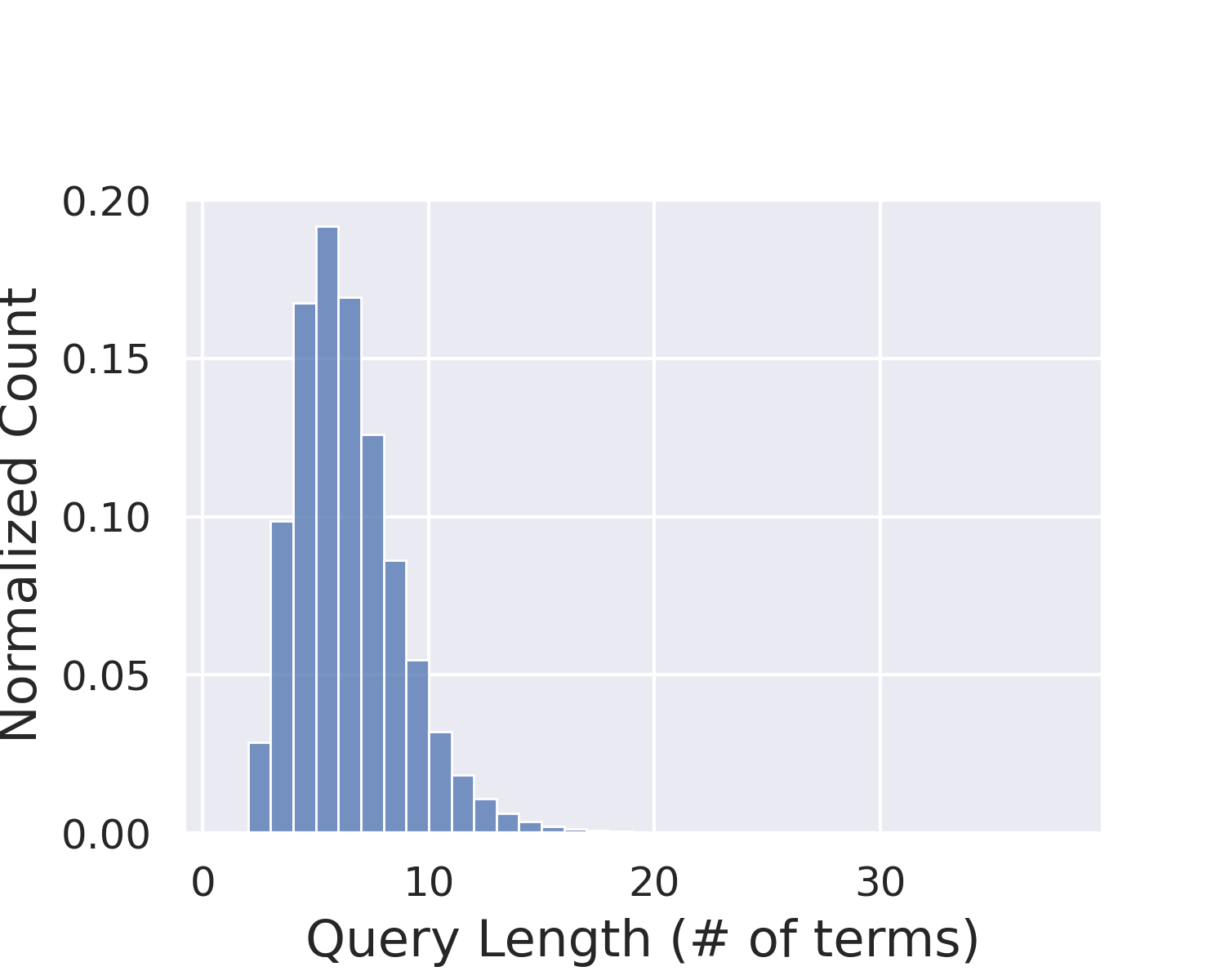
Fig. 23.1 Query length and document length distribution in Ad-hoc retrieval example using MS MARCO dataset.

There have been decades’ research and engineering efforts on developing ad-hoc retrieval models and system. Traditional IR systems primarily rely on techniques to identify exact term matches between a query and a document and compute final relevance score between various weighting schemes. Such exact matching approach has achieved tremendous success due to scalability and computational efficiency - fetching a handful of relevant document from billions of candidate documents. Unfortunately, exact match often suffers from vocabulary mismatch problem where sentences with similar meaning but in different terms are considered not matched. Recent development of deep neural network approach [HHG+13], particularly Transformer based pre-trained large language models, has made great progress in semantic matching, or inexact match, by incorporating recent success in natural language understanding and generation. Recently, combining exact matching with semantic matching is empowering many IR and search products.

Fig. 23.2 Google search engine.

Fig. 23.3 Microsoft Bing search engine.

23.1.2. Open-domain Question Answering

Another application closely related IR is open-domain question answering (OpenQA), which has found a widespread adoption in products like search engine, intelligent assistant, and automatic customer service. OpenQA is a task to answer factoid questions that humans might ask, using a large collection of documents (e.g., Wikipedia, Web page, or collected document) as the information source. An OpenQA example is like

Q: What is the capital of China?

A: Beijing.

Contrast to Ad-hoc retrieval, instead of simply returning a list of relevant documents, the goal of OpenQA is to identify (or extract) a span of text that directly answers the user’s question. Specifically, for factoid question answering, the OpenQA system primarily focuses on questions that can be answered with short phrases or named entities such as dates, locations, organizations, etc.

A typical modern OpenQA system adopts a two-stage pipeline [CFWB17] [Fig. 23.4]: (1) A document retriever selects a small set of relevant passages that probably contain the answer from a large-scale collection; (2) A document reader extracts the answer from relevant documents returned by the document retriever. Similar to ad-hoc search, relevant documents are required to be not only topically related to but also correctly address the question, which requires more semantics understanding beyond exact term matching features. One widely adopted strategy to improve OpenQA system with large corpus is to use an efficient document (or paragraph) retrieval technique to obtain a few relevant documents, and then use an accurate (yet expensive) reader model to read the retrieved documents and find the answer.

Nowadays many web search engines like Google and Bing have been evolving towards higher intelligence by incorporating OpenQA techniques into their search functionalities.

Fig. 23.4 A typical open-domain architecture where a retriever retrieves passages from information source relevant to the question.

Compared with ad-hoc retrieval, OpenQA shows reduced heterogeneity between the question and the answer passage/sentence yet add challenges of precisely understanding the question and locating passages that might contain answers. On one hand, the question is usually in natural language, which is longer than keyword queries and less ambiguous in intent. On the other hand, the answer passages/sentences are usually much shorter text spans than documents, leading to more concentrated topics/semantics. Retrieval and reader models need to capture the patterns expected in the answer passage/sentence based on the intent of the question, such as the matching of the context words, the existence of the expected answer type, and so on.

23.1.3. Modern IR Systems

A traditional IR system, or concretely a search engine, operates through several key steps.

The first step is crawling. A web search engines discover and collect web pages by crawling from site to site; Another vertical search engines such as e-commerce search engines collect their product information from product description and other product meta data. The second step is indexing, which creates an inverted index that maps key words to document ids. The last step is searching. Searching is a process that accepts a text query as input, looks up relevant documents from the inverted index, ranks documents, and returns a list of results, ranked by their relevance to the query.

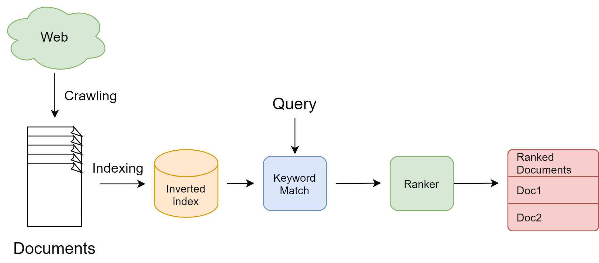
Fig. 23.5 Key steps in a traditional IR system.

The rapid progress of deep neural network learning [GBCB16] and their profound impact on natural language processing has also reshaped IR systems and brought IR into a deep learning age. Deep neural networks (e.g., Transformers [DCLT18]) have proved their unparalleled capability in semantic understanding over traditional IR margin yet they suffer from high computational cost and latency. This motivates the development of multi-stage retrieval and ranking IR system [Fig. 23.6] in order to better balance trade-offs between effectiveness (i.e., quality and accuracy of final results) and efficiency (i.e., computational cost and latency).

In this multi-stage pipeline, early stage models consists of simpler but more efficient models to reduce the candidate documents from billions to thousands; later stage models consists of complex models to perform accurate ranking for a handful of documents coming from early stages.

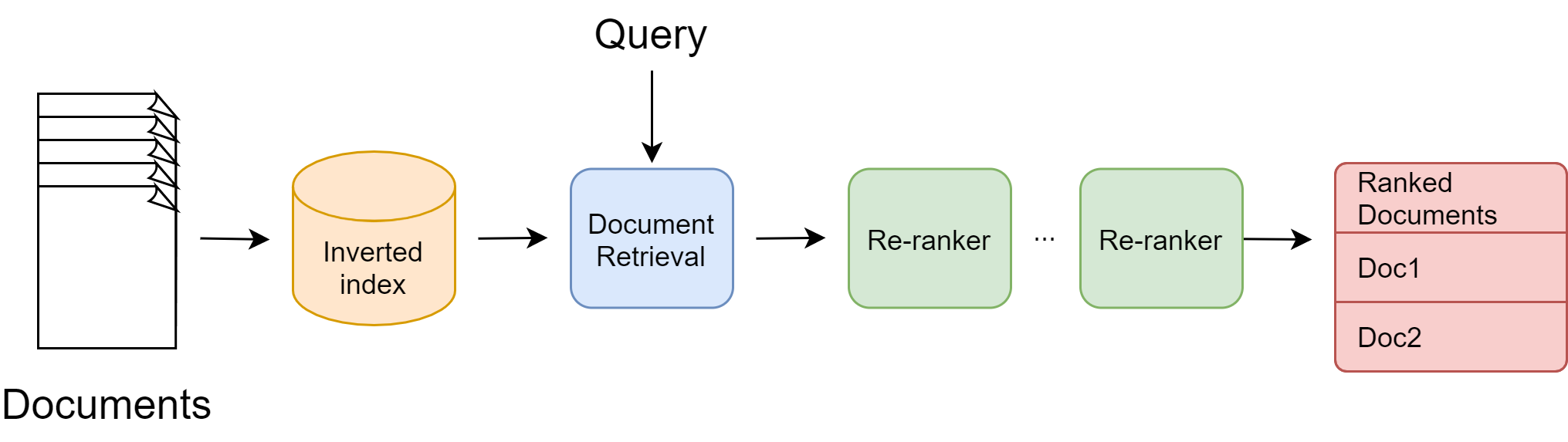
Fig. 23.6 The multi-stage architecture of modern information retrieval systems.

In modern search engine, traditional IR models, which is based on term matching, serve as good candidates for early stage model due to their efficiency. The core idea of the traditional approach is to count repetitions of query terms in the document. Large counts indicates higher relevance. Different transformation and weighting schemes for those counts lead to a variety of possible TF-IDF ranking features.

Later stage models are primarily deep learning model. Deep learning models in IR not only provide powerful representations of textual data that capture word and document semantics, allowing a machine to better under queries and documents, but also open doors to multi-modal (e.g., image, video) and multilingual search, ultimately paving the way for developing intelligent search engines that deliver rich contents to users.

Remark 23.1 (Why we need a semantic understanding model)

For web-scale search engines like Google or Bing, typically a very small set of popular pages that can answer a good proportion of queries.[MNCC16] The vast majority of queries contain common terms. It is possible to use term matching between key words in URL or title and query terms for text ranking; It is also possible to simply memorize the user clicks between common queries between their ideal URLs. For example, a query CNN is always matched to the CNN landing page. These simple methods clearly do not require a semantic understanding on the query and the document content.

However, for new or tail queries as well as new and tail document, a semantic understanding on queries and documents is crucial. For these cases, there is a lack of click evidence between the queries and the documents, and therefore a model that capture the semantic-level relationship between the query and the document content is necessary for text ranking.

23.1.4. Challenges And Opportunities In IR Systems

23.1.4.1. Query Understanding And Rewriting

A user’s query does not always have crystal clear description on the information need of the user. Rather, it often comes with potentially misspellings and unclear intent, and is usually very short, ranging from a few words to a few sentences [ch:neural-network-and-deep-learning:ApplicationNLP_IRSearch:tab:example_queries_MSMARCO]. There are several challenges to understand the user’s query.

Users might use vastly different query representations even though they have the same search intent. For example, suppose users like to get information about distance between Sun and Earth. Common used queries could be

• how far earth sun

• distance from sun to earth

• distance of earth from sun

• how far earth is from the sun

We can see that some of them are just key words rather than a full sentence and some of them might not have the completely correct grammar.

There are also more challenging scenarios where queries are often poorly worded and far from describing the searcher’s actual information needs. Typically, we employ a query rewriting component to expand the search and increase recall, i.e., to retrieve a larger set of results, with the hope that relevant results will not be missed. Such query rewriting component has multiple sub-components which are summarized below.

Spell checker Spell checking queries is an important and necessary feature of modern search. Spell checking enhance user experience by fixing basic spelling mistakes like itlian restaurat to italian restaurant.

Query expansion Query expansion improves search result retrieval by adding or substituting terms to the user’s query. Essentially, these additional terms aim to minimize the mismatch between the searcher’s query and available documents. For example, the query italian restaurant, we can expand restaurant to food or cuisine to search all potential candidates.

Query relaxation The reverse of query expansion is query relaxation, which expand the search scope when the user’s query is too restrictive. For example, a search for good Italian restaurant can be relaxed to italian restaurant.

Query intent understanding This subcomponent aims to figure out the main intent behind the query, e.g., the query coffee shop most likely has a local intent (an interest in nearby places) and the query earthquake may have a news intent. Later on, this intent will help in selecting and ranking the best documents for the query.

Given a rewritten query, It is also important to correctly weigh specific terms in a query such that we can narrow down the search scope. Consider the query NBA news, a relevant document is expected to be about NBA and news but have more focus on NBA. There are traditional rule-based approach to determine the term importance as well as recent data-driven approach that determines the term importance based on sophisticated natural language and context understanding.

To improve relevance ranking, it is often necessary to incorporate additional context information (e.g., time, location, etc.) into the user’s query. For example, when a user types in a query coffee shop, retrieve coffee shops by ascending distance to the user’s location can generally improve relevance ranking. Still, there are challenges on deciding for which type of query we need to incorporate the context information.

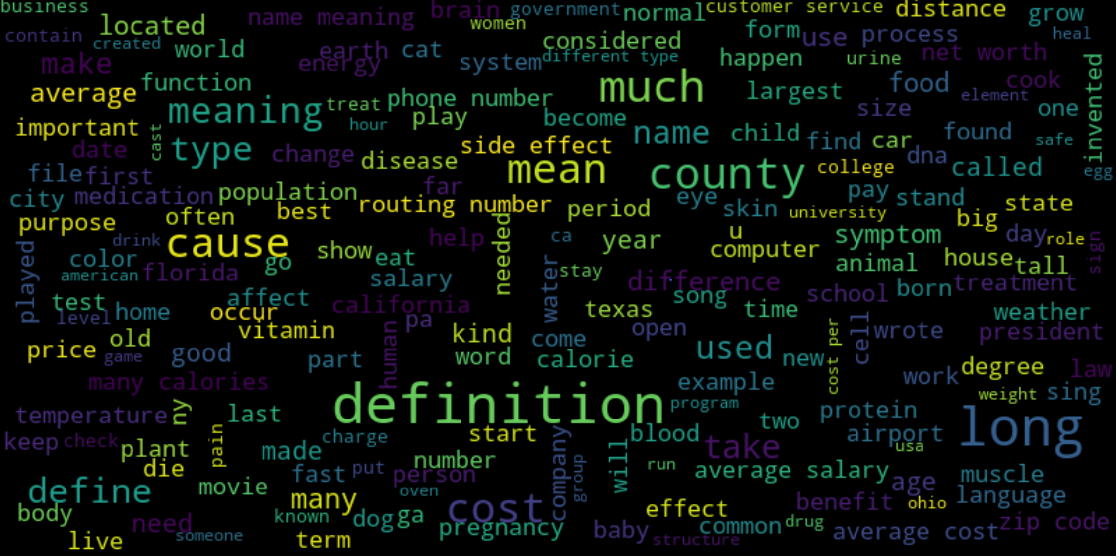
Fig. 23.7 Word cloud visualization for common query words using MS MARCO data.

23.1.4.2. Exact Match And Semantic Match

Traditional IR systems retrieve documents mainly by matching keywords in documents with those in search queries. While in many cases exact term match naturally ensure semantic match, there are cases, exact term matching can be insufficient.

The first reason is due to the polysemy of words. That is, a word can mean different things depending on context. The meaning of book is different in text book and book a hotel room. Short queries particularly suffer from Polysemy because they are often devoid of context.

The second reason is due to the fact that a concept is often expressed using different vocabularies and language styles in documents and queries. As a result, such a model would have difficulty in retrieving documents that have none of the query terms but turn out to be relevant.

Modern neural-based IR model enable semantic retrieval by learning latent representations of text from data and enable document retrieval based on semantic similarity.

Table 23.1 Retrieval results based on exact matching methods and semantic matching methods.

Query	“Weather Related Fatalities”
Information Need	A relevant document will report a type of weather event which has directly caused at least one fatality in some location.
Lexical Document	“.. Oklahoma and South Carolina each recorded three fatalities. There were two each in Arizona, Kentucky, Missouri, Utah and Virginia. Recording a single lightning death for the year were Washington, D.C.; Kansas, Montana, North Dakota, ..”
Semantic Document	.. Closed roads and icy highways took their toll as at least one motorist was killed in a 17-vehicle pileup in Idaho, a tour bus crashed on an icy stretch of Sierra Nevada interstate and 100-car string of accidents occurred near Seattle …

An IR system solely rely on semantic retrieval is vulnerable to queries that have rare words. This is because rare words are infrequent or even never appear in the training data and learned representation associated with rare words query might be poor due to the nature of data-driven learning. On the other hand, exact matching approach are robust to rare words and can precisely retrieve documents containing rare terms.

Another drawback of semantic retrieval is high false positives: retrieving documents that are only loosely related to the query.

Nowadays, much efforts have been directed to achieve a strong and intelligent modern IR system by combining exact match and semantic match approaches in different ways. Examples include joint optimization of hybrid exact match and semantic match systems, enhancing exact match via semantic based query and document expansion, etc.

23.1.4.3. Robustness To Document Variations

In response to users’ queries and questions, IR systems needs to search a large collection of text documents, typically at the billion-level scale, to retrieve relevant ones. These documents are comprised of mostly unstructured natural language text, as compared to structured data like tables or forms.

Documents can vary in length, ranging from sentences (e.g., searching for similar questions in a community question answering application like Quora) to lengthy web pages. A long document might like a short document, covering a similar scope but with more words, which is also known as the Verbosity hypothesis. On the other hand, a long document might consist of a number of unrelated short documents concatenated together, which is known as Scope hypothesis. The wide variation of document forms lead to different strategies. For example, following the Verbosity hypothesis a long document is represented by a single feature vector. Following the Scope hypothesis, one can break a long document into several semantically distinctive parts and represent each of them as separate feature vectors. We can consider each part as the unit of retrieval or rank the long document by aggregating evidence across its constituent parts.
For full-text scientific articles, we might choose to only consider article titles and abstracts, and ignoring most of the numerical results and analysis.

There are also challenges on breaking a long document into semantically distinctive parts and encode each part into meaningful representation. Recent neural network methods extract semantic parts by clustering tokens in the hidden space and represent documents by multi-vector representations[HSLW19, LETC21, TSJ+21].

23.1.4.4. Computational Efficiency

IR product such as search engines often serve a huge pool of user and need to handle tremendous volume of search requests during peak time (e.g., when there is breaking news events). To provide the best user experience, computational efficiency of IR models often directly affect user perceived latency. A long standing challenge is to achieve high accuracy/relevance in fetched documents yet to maintain a low latency. While traditional IR methods based on exact term match has excellent computational efficiency and scalability, it suffers from low accuracy due to the vocabulary and semantic mismatch problems. Recent progress in deep learning and natural language process are highlighted by complex transformer-based model [DCLT18] that achieved accuracy gain over traditional IR by a large margin yet experienced high latency issues. There are numerous ongoing studies (e.g., [GDC21, MC19, MDC17]) aiming to bring the benefits from the two sides via hybrid modeling methodology.

To alleviate the computational bottleneck from deep learning based dense retrieval, state-of-the-art search engines also adopts a multi-stage retrieval pipeline system: an efficient first-stage retriever uses a query to fetch a set of documents from the entire document collection, and subsequently one or more more powerful retriever to refine the results.

23.2. Text Ranking Evaluation Metrics

Consider a large corpus containing \(N\) documents \(D=\{d_1,...,d_N\}\). Given a query \(q\), suppose the retriever and its subsequent re-ranker (if there is) ultimately produce an ordered list of \(k\) relevant document \(R_q = \{d_{i_1},...,d_{i_k}\}\), where documents \(d_{i_1},...,d_{i_k} \) are ranked by some relevance measure with respect to the query.

In the following, we discuss several commonly used metrics to evaluate text ranking quality and IR system.

23.2.1. Precision And Recall

Precision and recall are metrics concerns the fraction of relevant documents retrieved for a query \(q\), but they are not concerned with the ranking order. Specifically, precision computes the fraction of relevant documents with respect to the total number of documents in the retrieved set \(R_{q}\), where \(R_{q}\) have \(K\) documents; Recall computes the fraction of relevant documents with respect to the total number of relevant documents in the corpus \(D\). More formally, we have

\[\begin{split}\begin{align*} \operatorname{Precision}_{q}@K &=\frac{\sum_{d \in R_{q}} \operatorname{rel}_{q}(d)}{\left|R_{q}\right|} = \frac{1}{K} \sum_{d \in R_{q}} \operatorname{rel}_{q}(d)\\ \operatorname{Recall}_{q}@K &=\frac{\sum_{d \in R_{q}} \operatorname{rel}_{q}(d)}{\sum_{d \in D} \operatorname{rel}_{q}(d)} \end{align*}\end{split}\]

where \(\operatorname{rel}_{q}(d)\) is a binary indicator function indicating if document \(d\) is relevant to \(q\). Note that the denominator \(\sum_{d \in D} \operatorname{rel}_{q}(d)\) is the total number of relevant documents in \(D\), which is a constant.

Typically, we only retrieve a fixed number \(K\) of documents, i.e., \(|R_q| = K\), where \(K\) typically takes 100 to 1000. The precision and recall at a given \(K\) can be computed over the total number of queries \(Q\), that is

\[\begin{split}\begin{align*} \operatorname{Precision}@{K} &=\frac{1}{|Q|}\sum_{q\in Q} \operatorname{Precision}_{q}@K \\ \operatorname{Recall}@{K} &=\frac{1}{|Q|}\sum_{q\in Q} \operatorname{Recall}_{q}@K \end{align*}\end{split}\]

Because recall has a fixed denominator, recall will increase as \(K\) increases.

23.2.2. Normalized Discounted Cumulative Gain (NDCG)

When we are evaluating retrieval and ranking results based on their relevance to the query, we normally evaluate the ranking result in the following way

• The ranking result is good if documents with high relevance appear in the top several positions in search engine result list.

• We expect documents with different degree of relevance should contribute to the final ranking in proportion to their relevance.

Cumulative Gain (CG) is the sum of the graded relevance scores of all documents in the search result list. CG only considers the relevance of the documents in the search result list, and does not consider the position of these documents in the result list. Given the ranking position of a result list, CG can be defined as:

\[CG@k = \sum_{i=1}^k s_i\]

where \(s_i\) is the relevance score, or custom defined gain, of document \(i\) in the result list. The relevance score of a document is typically provided by human annotators.

Discounted cumulative gain (DCG) is the discounted version of CG. The gain is accumulated from the top of the result list to the bottom, with the gain of each result discounted at lower ranks.

The traditional formula of DCG accumulated at a particular rank position \(k\) is defined as

\[ DCG@k=\sum_{i=1}^{k} \frac{s_{i}}{\log_{2}(i+1)}=s_{1}+\sum_{i=2}^{k} \frac{s_{i}}{\log _{2}(i+1)}. \]

An alternative formulation of \(DCG\) places stronger emphasis on more relevant documents:

\[ {DCG}@k=\sum_{i=1}^{p} \frac{2^{rel_q(d_i)}-1}{\log _{2}(i+1)}. \]

The ideal DCG, IDCG, is computed the same way but by sorting all the candidate documents in the corpus by their relative relevance so that it produces the max possible DCG@k. The normalized DCG, NDCG, is then given by,

\[ NDCG@k=\frac{DCG@k}{IDCG@k}. \]

Example 23.1

Consider 5 candidate documents with respect to a query. Let their ground truth relevance scores be

\[s_1=10, s_2=0,s_3=0,s_4=1,s_5=5,\]

which corresponds to a perfect rank of $\(s_1, s_5, s_4, s_2, s_3.\)\( Let the predicted scores be \)\(y_1=0.05, y_2=1.1, y_3=1, y_4=0.5, y_5=0.0,\)\( which corresponds to rank \)\(s_2, s_3, s_4, s_1, s_5.\)$

For \(k=1,2\), we have

\[DCG@k = 0, NDCG@k=0.\]

For \(k=3\), we have

\[DCG@k = \frac{s_4}{\log_2 (3+1)} = 0.5, IDCG@k = 10.0 + \frac{5.0}{\log_2 3} + \frac{1.0}{\log_2 4} = 13.65, NDCG@k=0.0366.\]

For \(k=4\), we have

\[DCG@k = \frac{s_4}{\log_2 4} + \frac{s_1}{\log_2 5} = 4.807, IDCG@k = IDCG@3 + 0.0 = 13.65, NDCG@k=0.352.\]

23.2.3. Online Metrics

When a text ranking model is deployed to serve user’s request, we can also measure the model performance by tracking several online metrics.

Click-through rate and dwell time When a user types a query and starts a search session, we can measure the success of a search session on user’s reactions. On a per-query level, we can define success via click-through rate. The Click-through rate (CTR) measures the ratio of clicks to impressions.

\[\operatorname{CTR} = \frac{\text{Number of clicks}}{\text{Number of impressions}},\]

where an impression means a page displayed on the search result page a search engine result page and a click means that the user clicks the page.

One problem with the click-through rate is we cannot simply treat a click as the success of document retrieval and ranking. For example, a click might be immediately followed by a click back as the user quickly realizes the clicked doc is not what he is looking for. We can alleviate this issue by removing clicks that have a short dwell time.

Time to success: Click-through rate only considers the search session of a single query. In real application case, a user’s search experience might span multiple query sessions until he finds what he needs. For example, the users initially search action movies and they do not find that the ideal results and refine the initial query to a more specific one: action movies by Jackie Chan. Ideally, we can measure the time spent by the user in identifying the page he wants as a metrics.

23.3. Traditional Sparse IR Fundamentals

23.3.1. Exact Match Framework

Most traditional approaches to ad-hoc retrieval simply count repetitions of the query terms in the document text and assign proper weights to matched terms to calculate a final matching score. This framework, also known as exact term matching, despite its simplicity, serves as a foundation for many IR systems. A variety of traditional IR methods fall into this framework and they mostly differ in different weighting (e.g., tf-idf) and term normalization (e.g., dogs to dog) schemes.

In the exact term matching, we represent a query and a document by a set of their constituent terms, that is, \(q = \{t^{q}_1,...,t^q_M\}\) and \(d = \{t^{d}_1,...,t^d_M\}\). The matching score between \(q\) and \(d\) with respect to a vocabulary \(V\) is given by:

\[ S(q, d)= \sum_{t\in V} f(t)\cdot\mathbb{1}(t\in q\cap d) = \sum_{t \in q \cap d} f(t) \]

where \(f\) is some function of a term and its associated statistics, the three most important of which are

• Term frequency (how many times a term occurs in a document);

• Document frequency (the number of documents that contain at least once instance of the term);

• Document length (the length of the document that the term occurs in).

Exact term match framework estimates document relevance based on the count of only the query terms in the document. The position of these occurrences and relationship with other terms in the document are ignored.

BM25 are based on exact matching of query and document words, which limits the in- formation available to the ranking model and may lead to problems such vocabulary mismatch

23.3.2. TF-IDF Vector Space Model

In the vector space model, we represent each query or document by a vector in a high dimensional space. The vector representation has the dimensionality equal to the vocabulary size, and in which each vector component corresponds to a term in the vocabulary of the collection. This query vector representation stands in contrast to the term vector representation of the previous section, which included only the terms appearing in the query. Given a query vector and a set of document vectors, one for each document in the collection, we rank the documents by computing a similarity measure between the query vector and each document

The most commonly used similarity scoring function for a document vector \(\vec{d}\) and a query vector \(\vec{q}\) is the cosine similarity \(\operatorname{Sim}(\vec{d}, \vec{q})\) is computed as

\[ \operatorname{Sim}(\vec{d}, \vec{q})=\frac{\vec{d}}{|\vec{d}|} \cdot \frac{\vec{q}}{|\vec{q}|}. \]

The component value associated with term \(t\) is typically the product of term frequency \(tf(t)\) and inverse document frequency \(idf(t)\). In addition, cosine similarity has a length normalization component that implicitly handles issues related to document length.

Over the years there have been a number of popular variants for both the TF and the IDF functions been proposed and evaluated. A basic version of \(tf(t)\) is given by

\[\begin{split} tf(t,d)= \begin{cases}\log \left(f_{t, d}\right)+1 & \text { if } f_{t, d}>0 \\ 0 & \text { otherwise. }\end{cases} \end{split}\]

where \(f_{t, d}\) is the actual term frequency count of \(t\) in document \(d\). Here the basic intuition is that a term appearing many times in a document should be assigned a higher weight for that document, and the its value should not necessarily increase linearly with the actual term frequency \(f_{t, d}\), hence the logarithm is used to proxy the saturation effect. Although two occurrences of a term should be given more weight than one occurrence, they shouldn’t necessarily be given twice the weight.

A common \(idf(t)\) functions is given by

\[ idf(t)=\log \left(N / N_{t}\right) \]

where \(N_t\) is the number of documents in the corpus that contain the term \(t\) and \(N\) is the total number of documents. Here the basic intuition behind the \(idf\) functions is that a term appearing in many documents should be assigned a lower weight than a term appearing in few documents.

23.3.3. BM25

One of the most widely adopted exact matching method is called BM25 (short for Okapi BM25)[CMS10, RZ09, YFL18]. BM25 combines overlapping terms, term-frequency (TF), inverse document frequency (IDF), and document length into following formula

\[ BM25(q, d)=\sum_{t_{q} \in q\cap d} i d f\left(t_{q}\right) \cdot \frac{t f\left(t_{q}, d\right) \cdot\left(k_{1}+1\right)}{t f\left(t_{q}, d\right)+k_{1} \cdot\left(1-b+b \cdot \frac{|d|}{a v g d l}\right)} \]

where \(tf(t_q, d)\) is the query’s term frequency in the document \(d\), \(|d|\) is the length (in terms of words) of document \(d\), \(avgdl\) is the average length of documents in the collection \(D\), and \(k_{1}\) and \(b\) are parameters that are usually tuned on a validation dataset. In practice, \(k_{1}\) is sometimes set to some default value in the range \([1.2,2.0]\) and \(b\) as \(0.75\). The \(i d f(t)\) is computed as,

\[ idf(t)=\log \frac{N-N_t+0.5}{N_t+0.5} \Leftarrow \log \frac{\text{Number of documents}}{\text{Number of documents with term } t}. \]

At first sight, BM25 looks quite like a traditional \(tf\times idf\) weight - a product of two components, one based on \(tf\) and one on \(idf\). Intuitively, a document \(d\) has a higher BM25 score if

• Many query terms also frequently occur in the document;

• These frequent co-occurring terms have larger idf values (i.e., they are not common terms).

However, there is one significant difference. The \(tf\) component in the BM25 uses some saturation mechanism to discount the impact of frequent terms in a document when the document length is long.

BM25 does not concerns with word semantics, that is whether the word is a noun or a verb, or the meaning of each word. It is only sensitive to word frequency (i.e., which are common words and which are rare words), and the document length. If one query contains both common words and rare words, this method puts more weight on the rare words and returns documents with more rare words in the query. Besides, a term saturation mechanism is applied to decrease the matching signal when a matched word appears too frequently in the document. A document-length normalization mechanism is used to discount term weight when a document is longer than average documents in the collection.

More specifically, two parameters in BM25, \(k_1\) and \(b\), are designed to perform term frequency saturation and document-length normalization,respectively.

• The constant \(k_{1}\) determines how the \(tf\) component of the term weight changes as the frequency increases. If \(k_{1}=0\), the term frequency component would be ignored and only term presence or absence would matter. If \(k_{1}\) is large, the term weight component would increase nearly linearly with the frequency.

• The constant \(b\) regulates the impact of the length normalization, where \(b=0\) corresponds to no length normalization, and \(b=1\) is full normalization.

Remark 23.2 (Weighting scheme for long queries)

If the query is long, then we might also use similar weighting for query terms. This is appropriate if the queries are paragraph-long information needs, but unnecessary for short queries.

\[ BM25(q, d)=\sum_{t_q \in q\cap d} idf(t_q) \cdot \frac{\left(k_{1}+1\right) tf(t_q,d) }{k_{1}\left((1-b)+b \times |d|/avgdl\right)+tf(t_q,d)} \cdot \frac{\left(k_{3}+1\right) tf(t_q,q)}{k_{2}+tf(t_q,q)} \]

with \(tf(t_q, q)\) being the frequency of term \(t\) in the query \(q\), and \(k_{2}\) being another positive tuning parameter that this time calibrates term frequency scaling of the query.

23.3.4. BM25 Efficient Implementation

To efficient implementation of BM25, we can pre-compute document side term frequency and store it, which is known as Eager indexing-time scoring process [Lu24]. This includes:

• Tokenize each document into tokens

• Compute the number of documents containing each token and token frequency in each document.

• Compute the idf for each token using the document frequencies

• Compute the BM25 scores for each token in each document \(BM25(t_i,d)\)

During the query process, we tokenize the query \(q\) into tokens \(t_i\) and compute

\[BM25(q, d) = \sum_{t_i \in q\cap d} BM25(t_i,d).\]

23.3.5. BM25F

[RZ09]

23.4. Query and Document Expansion

23.4.1. Overview

Query expansion and document expansion techniques provide two potential solutions to the inherent vocabulary mismatch problem in traditional IR systems. The core idea is to add extra relevant terms to queries and documents respectively to aid relevance matching.

Consider an ad-hoc search example of automobile sales per year in the US.

• Document expansion can be implemented by appending car in documents that contains the term automobile but not car. Then an exact-match retriever can fetch documents containing either car and automobile.

• Query expansion can be accomplished by retrieving results from both the query automobile sales per year in the US and the query car sales per year in the US.

There are many different approaches to coming up suitable terms to expand queries and documents in order to make relevance matching easier. These approaches range from traditional rule-based methods such as synonym expansion to recent learning based approaches by mining user logs. For example, augmented terms for a document can come from queries that are relevant from user click-through logs.

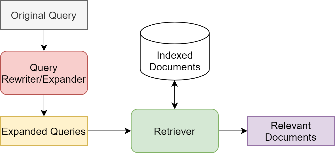
Fig. 23.8 Query expansion module in an IR system.

Both query and document expansion can be fit into typical IR architectures through an de-coupled module. A query expansion module takes an input query and output a (richer) expanded query [Fig. 23.8]. They are also known as query rewriters or expanders. The module might remove terms deemed unnecessary in the user’s query, for example stop words and add extra terms facilitate the engine to retrieve documents with a high recall.

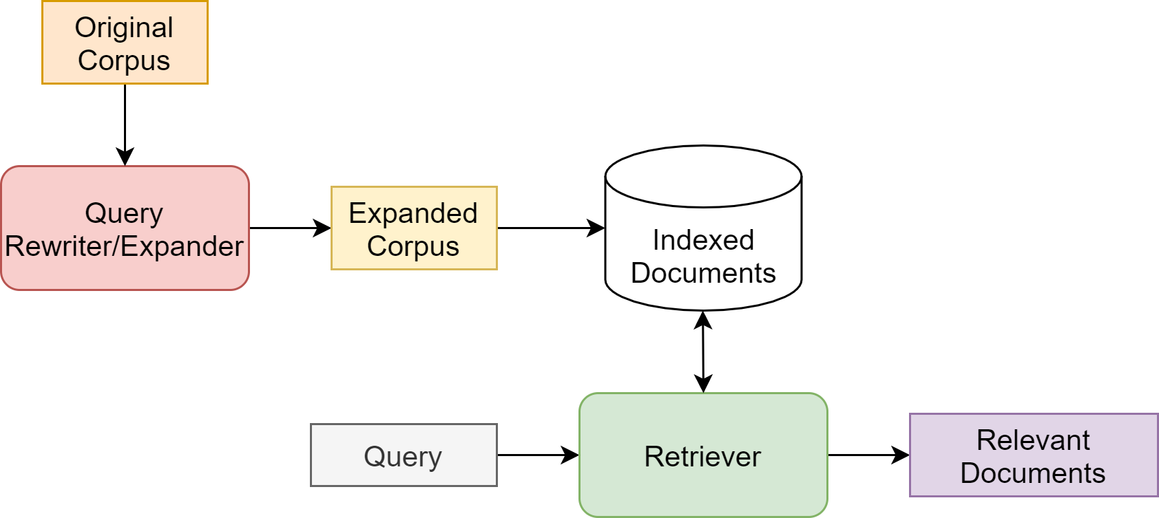
Fig. 23.9 Document expansion module in an IR system.

Similarly, document expansion naturally fits into the retrieval and ranking pipeline [Fig. 23.9]. The index will be simply built upon the expanded corpus to provide a richer set of candidate documents for retrieval. The extra computation for document expansion can be all carried out offline. Therefore, it presents the same level of effectiveness like query expansion but at lower latency costs (for example, using less computationally intensive rerankers).

Query expansion and document expansion have different pros and cons. Main advantages of query expansions include

• Compare to document expansion, query expansion techniques can be quickly implemented and experimented without modifying the entire indexing. On the other hand, experimenting document expansion techniques can be costly and time-consuming, since the entire indexing is affected.

• Query expansion techniques are generally more flexible. For example, it is easy to switch on or off different features at query time (for example, selectively apply expansion only to certain intents or certain query types). The flexibility of query expansion also allow us insert an expansion module in different stages of the retrieval-ranking pipeline.

On the other hand, one unique advantage for document expansion is that: documents are typically much longer than queries, and thus offer more context for a model to choose appropriate expansion terms. Neural based natural language generation models, like Transformers [VSP+17], can benefit from richer contexts and generate cohesive natural language terms to expand original documents.

23.4.2. Document Expansion via Query Prediction

Authors in [NYLC19] proposed DocT5Query, a document expansion strategy based on a seq-to-seq natural language generation model to enrich each document.

For each document, the transformer generation model predicts a set of queries that are likely to be relevant to the document. Given a dataset of (query, relevant document) pairs, we use a transformer model is trained to takes the document as input and then to produce the target query^{[^3]}.

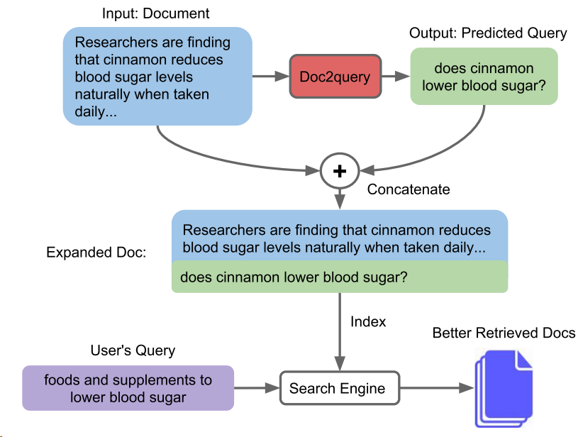
Fig. 23.10 Given a document, our Doc2query model predicts a query, which is appended to the document. Expansion is applied to all documents in the corpus, which are then indexed and searched as before. Image from [NYLC19].

Once the model is trained, we can use the model to predict top-\(k\) queries using beam search and append them to each document in the corpus.

Examples of query predictions on MS MARCO compared to real user queries.

• Input Document: July is the hottest month in Washington DC with an average temperature of 80F and the coldest is January at 38F with the most daily sunshine hours at 9 in July. The wettest month is May with an average of \(100 \mathrm{ mm}\) of rain.

• Predicted Query: weather in washington dc

• Target Query: what is the temperature in washington

Another example:

• Input Document: sex chromosome - (genetics) a chromosome that determines the sex of an individual; mammals normally have two sex chromosomes chromosome - a threadlike strand of DNA in the cell nucleus that carries the genes in a linear order; humans have 22 chromosome pairs plus two sex chromosomes.

• Predicted Query: what is the relationship between genes and chromosomes

• Target Query: *which chromosome controls sex characteristics *

This document expansion technique has demonstrated its effectiveness on the MS MARCO dataset when it is combined with BM25. The query prediction improves the performance from two aspects:

• Predicted queries tend to copy some words from the input document (e.g., Washington DC, chromosome), which is sort of equivalent to performing term re-weighting (i.e., increasing the importance of key terms).

• Predicted queries might also contain words not present in the input document (e.g., weather), which can be characterized as expansion by synonyms and other related terms.

A widely used relevance feedback algorithm was developed by Rocchio [Roc71] for vector space models. Let \(\left\{d_{1}, d_{2}, \cdots, d_{k}\right\}\) be the vectors top \(k\) documents retrieved by SNRM in response to the query vector \(q\). The updated query vector is computed as:

\[ \vec{q}^{*}=\vec{q}+\alpha \frac{1}{k} \sum_{i=1}^{k} \vec{d}_{i} \]

where \(\alpha\) controls the weight of the feedback vector. In practice we only keep the top \(t\) (e.g., \(t=10 -20\)) terms with the highest values in the updated query vector \(\vec{q}^{*}\).

A continued study in this line shows that replacing the transformer with more powerful seq-to-seq transformer model T5 [RSR+19] can bring further performance gain.

23.5. Contextualized Term Importance

23.5.1. Context-aware Term Importance: Deep-CT

In ad-hoc search, queries are mainly short and keyword based without complex grammatical structures. To be able to fetch most relevant results, it is important to take into account term importance. For example, given the query bitcoin news, a relevant document is expected to be about bitcoin and news, where the term bitcoin is more important than news in the sense that a document describing other aspects of bitcoin would be more relevant than a document describing news of other things.

In the traditional IR framework, term importance is calculated using inverse document frequency. A term is less important if it is a common term appearing in a large number of documents. These frequency-based term weights have been a huge success in traditional IR systems due to its simplicity and scalability. The problematic aspect is that Tf-idf determines the term importance solely based on word counts rather than the semantics. High-frequency words does not necessarily indicate their central role to the meaning of the text, especially for short texts where the word frequency distribution is quite flat. Considering the following two passages returned for the query stomach [DC19], one is relevant and one is not:

• Relevant: In some cases, an upset stomach is the result of an allergic reaction to a certain type of food. It also may be caused by an irritation. Sometimes this happens from consuming too much alcohol or caffeine. Eating too many fatty foods or too much food in general may also cause an upset stomach.

• Less relevant: All parts ofthe body (muscles , brain, heart, and liver) need energy to work. This energy comes from the food we eat. Our bodies digest the food we eat by mixing it with fluids( acids and enzymes) in the stomach. When the stomach digests food, the carbohydrate (sugars and starches) in the food breaks down into another type of sugar, called glucose.

In both passages, the word stomach appear twice; but the second passage is actually off-topic. This example also suggests that the importance of a term depends on its context, which helps understand the role of the word playing in the text.

Authors in [DC19] proposed DeepCT, which uses the contextual word representations from BERT to estimate term importance to improve the traditional IR approach. Specifically, given a word in a specific text, its contextualized word embedding (e.g., BERT) is used a feature vector that characterizes the word’s syntactic and semantic role in the text. Then DeepCT estimates the word’s importance score via a weighted summation: $\( \hat{y}_{t, c}= {w} T_{t, c}+b \)\( where \)T_{t, c} \in \mathbb{R}^D\( is token \)t\( 's contextualized embedding in the text \)c\(; and, \){w}\in \mathbb{R}^D\( and \)b$ are the weights and bias.

The model parameters of DeepCT are the weight and bias, and they can be estimated from a supervised learning task, per-token regression, given by $\( L_{MSE}=\sum_{c} \sum_{t}\left(y_{t, c}-\hat{y}_{t, c}\right)^{2}. \)$

The ground truth term weight \(y_{t, c}\) for every word in either the query or the document are estimated in the following manner.

• The importance of a term in a document \(d\) is estimated by the occurrence of the term in relevant queries [Fig. 23.11]. More formally, it is given by $\( QTR(t, d)=\frac{\left|Q_{d, t}\right|}{\left|Q_{d}\right|} \)\( \)Q_{d}\( is the set of queries that are relevant to document \)d\(. \)Q_{d, t}\( is the subset of \)Q_{d}\( that contains term \)t$. The intuition is that words that appear in relevant queries are more important than other words in the document.

• The importance of a term in a document \(d\) is estimated by the occurrence of the term in relevant queries [Fig. 23.11]. More formally, it is given by $\( TR(t, q)=\frac{\left|D_{q, t}\right|}{\left|D_{q}\right|} \)\( \)D_{q}\( is the set of documents that are relevant to the query \)q\(. \)D_{q, t}\( is the subset of relevant documents that contains term \)t$. The intuition is that a query term is more important if it is mentioned by more relevant documents.

Fig. 23.11 Illustration of calculating context-aware term importance for a query (left) and a document (right). Term importance in a query is estimated from relevant documents of the query; term importance in a document is estimated from relevant queries of the document.

23.5.1.1. Learnable Context-aware Term Importance: Deep-Impact

DeepCT has an interesting “quirk”: in truth, it only learns the term frequency (tf) component of term weights, but still relies on the remaining parts of the BM25 scoring function via the gen- eration of pseudo-documents. This approach also has a weakness: it only assigns weights to terms that are already present in the document, which limits retrieval to exact match. This is an impor- tant limitation that is addressed by the use of dense representations, which are capable of capturing semantic matches.

Deep CT learning independent term-level scores without taking into account the term co-occurrences in the document.

DeepCT (Dai and Callan, 2019), which uses a transformer to learn term weights based on a re- gression model, with the supervision signal coming from the MS MARCO passage ranking test collection

DeepImpact brought together two key ideas: the use of document expansion to iden- tify dimensions in the sparse vector that should have non-zero weights and a term weighting model based on a pairwise loss between relevant and non- relevant texts with respect to a query. Expansion

DeepImpact aim at learning the final term impact jointly across all query terms occurring in a passage. DeepImpact learns richer interaction patterns among the impacts, when compared to training each im- pact in isolation.

To address vocabulary mismatch, DeepImpact leverages DocT5Query to enrich every document with new terms likely to occur in queries for which the document is relevant.

Network architecture The overall architecture of the Deeplmpact neural network is depicted in Figure 1. Deeplmpact feeds a contextual LM encoder the original document terms (in white) and the injected expansion terms (in gray), separating both by a [SEP] separator token to distinguish both contexts. The LM encoder produces an embedding for each input term. The first occurrence of each unique term is provided as input to the impact score encoder, which is a two-layer MLP with ReLU activations. This produces a single-value positive score for each unique term in the document, representing its impact. Given a query \(q\), we model the score of document \(d\) as simply the sum of impacts for the intersection of terms in \(q\) and \(d\). That is, $\(s(q, d) = \sum_{t\in q\cap d} \operatorname{ScoreEncoder}(h_t).\)$

For each triple, two scores for the corresponding two documents are computed. The model is optimized via pairwise Softmax cross- entropy loss over the computed scores of the documents.

Fig. 23.12 DeepImpact architecture.

Quantization and Query Processing. In our approach we predict real-valued document-term scores, also called impact scores, that we store in the inverted index. Since storing a floating point value per posting would blow up the space requirements of the inverted index, we decided to store impacts in a quantized form. The quantized impact scores belong to the range of \(\left[1,2^{b}-1\right]\), where \(b\) is the number of bits used to store each value. We experimented with b = 8 using linear quantization, and did not notice any loss in precision w.r.t. the original scores.

23.5.2. TW-BERT

[SLK+23]

23.6. Sparse Retrieval Demonstrations

23.6.1. BM25 Demonstration

Consider a doc corpus consisting of the following documents.

DocID	Doc Text
0	Washington, D.C. (also known as simply Washington or D.C., and officially as the District of Columbia) is the capital of the United States. It is a federal district. The President of the USA and many major national government offices are in the territory. This makes it the political center of the United States of America.
1	Hammonton is a town in Atlantic County, New Jersey, United States, known as the “Blueberry Capital of the World.” As of the 2010 United States Census, the town’s population was 14,791.
2	Nevada is one of the United States’ states. Its capital is Carson City. Other big cities are Las Vegas and Reno.
3	‘Ohio is one of the 50 states in the United States. Its capital is Columbus. Columbus also is the largest city in Ohio.’
4	Capital punishment (the death penalty) has existed in the United States since before the United States was a country. As of 2017, capital punishment is legal in 30 of the 50 states. The federal government (including the United States military) also uses capital punishment.

Given the query What is the capital of the United States, which contains tokens {capital, united, states} after stopword removal, we can compute the following sorted list based on BM25 scores.

BM25 Score	Doc Text
0.164	Capital punishment (the death penalty) has existed in the United States since before the United States was a country. As of 2017, capital punishment is legal in 30 of the 50 States. The federal government (including the United States military) also uses capital punishment.
0.143	‘Ohio is one of the 50 States in the United States. Its capital is Columbus. Columbus also is the largest city in Ohio.’
0.139	Nevada is one of the United States’ states. Its capital is Carson City. Other big cities are Las Vegas and Reno.
0.131	Hammonton is a town in Atlantic County, New Jersey, United States, known as the “Blueberry capital of the World.” As of the 2010 United States Census, the town’s population was 14,791.
0.120	Washington, D.C. (also known as simply Washington or D.C., and officially as the District of Columbia) is the capital of the United States. It is a federal district. The President of the USA and many major national government offices are in the territory. This makes it the political center of the United States of America.

We have the following observations:

• The most relevant document (doc 0) has the lowest score due to the fact that

  • Document is long

  • The word capital appears once, united states appear twice

• The irrelevant document (doc 4) has the highest score due to the fact that words in {capital, united, states} appear multiple times.

In general BM25-based counting apporach cannot capture the semantic accurately and have a poor precision @ k and we need to rely on dense models like bi-encoder and cross-encoder.

Remark 23.3 (Stopword removal)

• In naive sparse retrieval, stopwords in the query and documents are directly dropped.

• Stopwords are usually coming from a curated word list and the determination of stopword is dependent on the word list creator. For example, in the sklearn.feature_extraction._stop_words, what and when are included as stopwords.

• In some queries, stopwords can be critical for the accurate interpretation of the query intent.

• Instead of naively removing all the stopwords, one can use contextualized term importance model to determine the importance of stopwords in the query (see Contextualized Term Importance).

For the same query, if we apply bi-encoder retrieval model (multi-qa-MiniLM-L6-cos-v1) to compute the similarity score with the corpus, we have the following scores.

The dense retriever is able to achieve semantic understanding the query and doc:

• Top 1 result is most relevant

• Top 2 and 3 results are weakly relevant

Biencoder Scores	Doc Text
0.57	Washington, D.C. (also known as simply Washington or D.C., and officially as the District of Columbia) is the capital of the United States. It is a federal district. The President of the USA and many major national government offices are in the territory. This makes it the political center of the United States of America.
0.49	‘Ohio is one of the 50 states in the United States. Its capital is Columbus. Columbus also is the largest city in Ohio.’
0.48	Nevada is one of the United States’ states. Its capital is Carson City. Other big cities are Las Vegas and Reno.
0.37	Capital punishment (the death penalty) has existed in the United States since before the United States was a country. As of 2017, capital punishment is legal in 30 of the 50 states. The federal government (including the United States military) also uses capital punishment.
0.18	Hammonton is a town in Atlantic County, New Jersey, United States, known as the “Blueberry Capital of the World.” As of the 2010 United States Census, the town’s population was 14,791.

Remark 23.4 (Sparse and dense retriever comparison)

In the above example, dense retriever shows a clear advantage over sparse retriever. However, the observation from BEIR benchmark is that BM25 remains as a stronger baseline compared to dense retriever across diverse domains. The seemingly contradictory results can be understood from the following results

• BM25 is usually performing poorly for short documents, where word count frequency are quite uniform across different words - in other words, two documents with different topics can have a similar count stats for the same query terms.

• Dense retriever model tend to have weaker performance over long documents and in tail topic domains.

  • Encoding a document into a fixed length vector (e.g., 512) will have more information loss for long documents due to context window limit (i.e., a model might truncate the part exceeding its max context length) or the model’s own capacity.

  • Tail topic (e.g., topics involve uncommon technical jargons) have a much lower presence in the training corpus, causing inferior semantic understanding of the topic.

Also see Discussion: Sparse and Dense Retrieval for a more detailed discussion.

23.7. Note on Bibliography and Software

23.7.1. Bibliography

For excellent reviews in neural information retrieval, see [GFP+20, LNY21, MC+18]

For traditional information retrieval, see [BCC16, CMS10, RZ09, SchutzeMR08]

[BCC16]

Stefan Buttcher, Charles LA Clarke, and Gordon V Cormack. Information retrieval: Implementing and evaluating search engines. Mit Press, 2016.

[CFWB17]

Danqi Chen, Adam Fisch, Jason Weston, and Antoine Bordes. Reading wikipedia to answer open-domain questions. arXiv preprint arXiv:1704.00051, 2017.

[CMS10] (1,2)

W Bruce Croft, Donald Metzler, and Trevor Strohman. Search engines: Information retrieval in practice. Volume 520. Addison-Wesley Reading, 2010.

[DC19] (1,2)

Zhuyun Dai and Jamie Callan. Context-aware sentence/passage term importance estimation for first stage retrieval. arXiv preprint arXiv:1910.10687, 2019.

[DCLT18] (1,2)

Jacob Devlin, Ming-Wei Chang, Kenton Lee, and Kristina Toutanova. Bert: pre-training of deep bidirectional transformers for language understanding. arXiv preprint arXiv:1810.04805, 2018.

[GDC21]

Luyu Gao, Zhuyun Dai, and Jamie Callan. Coil: revisit exact lexical match in information retrieval with contextualized inverted list. arXiv preprint arXiv:2104.07186, 2021.

[GBCB16]

Ian Goodfellow, Yoshua Bengio, Aaron Courville, and Yoshua Bengio. Deep learning. Volume 1. MIT press Cambridge, 2016.

[GFP+20]

Jiafeng Guo, Yixing Fan, Liang Pang, Liu Yang, Qingyao Ai, Hamed Zamani, Chen Wu, W Bruce Croft, and Xueqi Cheng. A deep look into neural ranking models for information retrieval. Information Processing & Management, 57(6):102067, 2020.

[HHG+13]

Po-Sen Huang, Xiaodong He, Jianfeng Gao, Li Deng, Alex Acero, and Larry Heck. Learning deep structured semantic models for web search using clickthrough data. In Proceedings of the 22nd ACM international conference on Information & Knowledge Management, 2333–2338. 2013.

[HSLW19]

Samuel Humeau, Kurt Shuster, Marie-Anne Lachaux, and Jason Weston. Poly-encoders: transformer architectures and pre-training strategies for fast and accurate multi-sentence scoring. arXiv preprint arXiv:1905.01969, 2019.

[LNY21]

Jimmy Lin, Rodrigo Nogueira, and Andrew Yates. Pretrained transformers for text ranking: bert and beyond. Synthesis Lectures on Human Language Technologies, 14(4):1–325, 2021.

[LETC21]

Yi Luan, Jacob Eisenstein, Kristina Toutanova, and Michael Collins. Sparse, dense, and attentional representations for text retrieval. Transactions of the Association for Computational Linguistics, 9:329–345, 2021.

[Lu24]

Xing Han Lù. Bm25s: orders of magnitude faster lexical search via eager sparse scoring. arXiv preprint arXiv:2407.03618, 2024.

[MC19]

Bhaskar Mitra and Nick Craswell. An updated duet model for passage re-ranking. arXiv preprint arXiv:1903.07666, 2019.

[MC+18]

Bhaskar Mitra, Nick Craswell, and others. An introduction to neural information retrieval. Now Foundations and Trends Boston, MA, 2018.

[MDC17]

Bhaskar Mitra, Fernando Diaz, and Nick Craswell. Learning to match using local and distributed representations of text for web search. In Proceedings of the 26th International Conference on World Wide Web, 1291–1299. 2017.

[MNCC16]

Bhaskar Mitra, Eric Nalisnick, Nick Craswell, and Rich Caruana. A dual embedding space model for document ranking. arXiv preprint arXiv:1602.01137, 2016.

[NYLC19] (1,2)

Rodrigo Nogueira, Wei Yang, Jimmy Lin, and Kyunghyun Cho. Document expansion by query prediction. arXiv preprint arXiv:1904.08375, 2019.

[RSR+19]

Colin Raffel, Noam Shazeer, Adam Roberts, Katherine Lee, Sharan Narang, Michael Matena, Yanqi Zhou, Wei Li, and Peter J Liu. Exploring the limits of transfer learning with a unified text-to-text transformer. arXiv preprint arXiv:1910.10683, 2019.

[RZ09] (1,2,3)

Stephen Robertson and Hugo Zaragoza. The probabilistic relevance framework: BM25 and beyond. Now Publishers Inc, 2009.

[Roc71]

Joseph Rocchio. Relevance feedback in information retrieval. The Smart retrieval system-experiments in automatic document processing, pages 313–323, 1971.

[SLK+23]

Karan Samel, Cheng Li, Weize Kong, Tao Chen, Mingyang Zhang, Shaleen Gupta, Swaraj Khadanga, Wensong Xu, Xingyu Wang, Kashyap Kolipaka, and others. End-to-end query term weighting. In Proceedings of the 29th ACM SIGKDD Conference on Knowledge Discovery and Data Mining, 4778–4786. 2023.

[SchutzeMR08]

Hinrich Schütze, Christopher D Manning, and Prabhakar Raghavan. Introduction to information retrieval. Volume 39. Cambridge University Press Cambridge, 2008.

[TSJ+21]

Hongyin Tang, Xingwu Sun, Beihong Jin, Jingang Wang, Fuzheng Zhang, and Wei Wu. Improving document representations by generating pseudo query embeddings for dense retrieval. arXiv preprint arXiv:2105.03599, 2021.

[VSP+17]

Ashish Vaswani, Noam Shazeer, Niki Parmar, Jakob Uszkoreit, Llion Jones, Aidan N Gomez, Łukasz Kaiser, and Illia Polosukhin. Attention is all you need. In Advances in neural information processing systems, 5998–6008. 2017.

[YFL18]

Peilin Yang, Hui Fang, and Jimmy Lin. Anserini: reproducible ranking baselines using lucene. Journal of Data and Information Quality (JDIQ), 10(4):1–20, 2018.

23.7.2. Software

Faiss is a recently developed computational library for efficient similarity search and clustering of dense vectors.