11. LLM Training Fundamentals

11.1. Training Overview

The chapter discuss LLM training, which can be broadly divided into two stages, each with its own purpose and methodologies:

1. Pretraining: This initial phase involves using self-supervised learning (e.g., autoregressive learning objective) let the model to learn language structures of a diverse and extensive corpus of text data. The model learns to predict words or tokens based on context, developing a broad understanding of language structure and semantics. We’ll discuss the basics of pretraining and explore the concept of continuing pretraining, which allows models to adapt to new domains or languages.

2. Post-training: After the initial pretraining, models often undergo additional training phases to enhance their performance on specific tasks or to better follow instructions. This includes:

   • Finetuning: Adapting the pretrained model to specific tasks or domains. Particularly, instruction finetuning involves teaching the model to follow explicit instructions or prompts by training on large-scale and diverse (instruction, response) pair data. We cover this in LLM Finetuning.

   • Alignment and Preference Learning: Ensuring the model’s outputs align with human values and preferences. we cover this direction in LLM Alignment and Preference Learning.

Finally, we cover fundamentals in LLM optimization algorithms. Throughout the LLM training process, various optimization algorithms are employed to adjust the model’s parameters efficiently. We’ll examine popular techniques such as stochastic gradient descent (SGD), Adam, and their variants, discussing how they contribute to the model’s learning process.

11.2. Pretraining Techniques

11.2.1. Next-Token Prediction (NTP)

Pretraining has become a cornerstone in the development of LLM, which contributes to

• the general langugae understand and generation ability

• acquire world knowledge

• other emergent abilities like reasoning

The dominant LLM pretraining objective is auto-regressive language modeling, which predict the next words given preceding word sequence. Given an input sequence \(\mathbf{x} = (x_1,...,x_T)\), auto-regressive language modeling minimize the negative log likelihood given by

\[L = - \sum_{t=1}^{T} \log p\left(x_{t} \mid \mathbf{x}_{t-k-1:t-1},\theta\right)\]

where \(p\left(x_{t} \mid \mathbf{x}_{t-k-1:t-1}\right)\) is the predicted probability distribution for token \(x_t\) given preceding token sequence \(\mathbf{x}_{t-k-1:t-1}\) with a context window size \(k\) (\(k\) can range from hundreds to tens of thousands, depending on the model configuration).

There are scaling laws [HKK+20, KMH+20] discovered on LLM pretraining, which establishes mathematical relationships model performance given model size, dataset size, and the amount of compute. The availability of scaling laws has several benefits:

• It provides to benchmark to enable LLM pretraining to be done in a predictable way.

• It help design better training strategy by optimizing the model size and data size under a compute budget.

11.2.2. Fill-in-the Middle (FIM)

Fill-in-the Middle (FIM)[BJT+22, LAZ+23] was proposed in as a technique used to improve the in-context learning and generalization capabilities of large language models (LLMs). Instead of always training the model to generate text in a left-to-right (causal) manner, FIM involves predicting a missing segment of text when given both the preceding and succeeding context.

Specifially, FIM training makes LLMs better at predicting missing code/text blocks and handling real-world coding and writing workflows:

• In coding applications (e.g., GitHub Copilot, OpenAI Codex), developers often insert code or docstring into existing structures rather than appending to the end;

• In writing and editting tasks, users need to insert or modify text within a document.

The implementation of FIM involves randomly dividing the text into three parts, then shuffling the order of these parts and connecting them with special characters. Depending on how the segments are ordered, there are two distinct modes: PSM (Prefix-Suffix-Middle) and SPM (Suffix-Prefix-Middle).

For example, in the SPM mode, the training corpus is transformed to

\[ <\text { <PRE> }> prefix <\text { SUF }> suffix <\text { MID }> middle \]

where \(<\text { <PRE> }>, <\text { SUF }>, <\text { MID }>\) are sentinel tokens.

During the inference where we would like to use prefix and surfix to predict the middle, we can prompt the model with

\[ <\text { <PRE> }> prefix <\text { SUF }> suffix <\text { MID }> middle \]

During pretraining, FIM and left-to-right autoregression can be both applied to the training corpus and then use the same NSP training task. And surpringly, FIM will not strongly compromise the left-to-right capability with high FIM rate up to 90%, and at the same time, the model acquires FIM ability for code and language (known as FIM-for-free property). The authors also suggested that 50% FIM rate strike a good balance. Practioners from [GZY+24] also used 50% FIM rate in the pretraining for coding LLM.

11.2.3. Multiple Token Prediction (MTP)

Besides training using a next-token prediction loss, there are efforts exploring training language models to predict multiple future tokens at once [GIRoziere+24]. More specifically, at each position in the training corpus, we ask the model to predict the following \(n\) tokens using \(n\) independent output heads, operating on top of a shared model trunk[Fig. 11.1].

This MTP scheme brings advantages:

• Higher sample efficiency during training.

• During inference, we can either use one next-token output head or optionally use the additional heads to speed up the inference time.

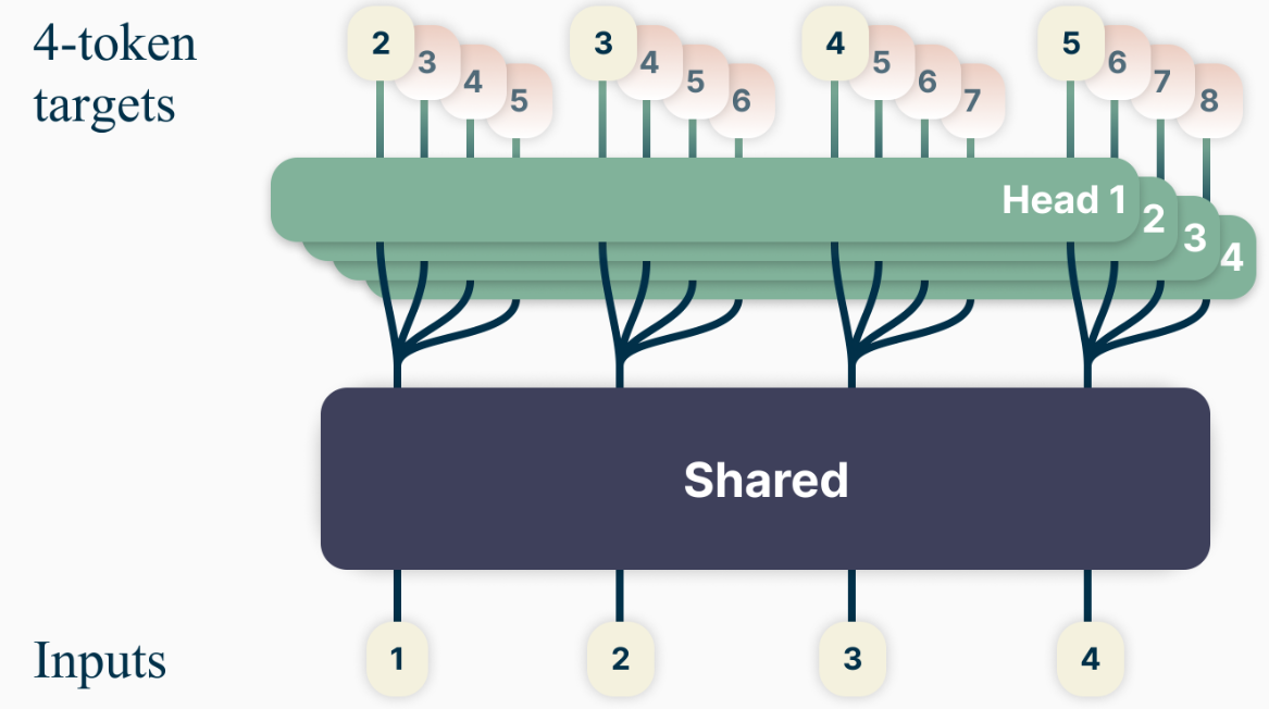
Fig. 11.1 Overview of multi-token prediction. During training, the model predicts 4 future tokens at once, by means of a shared trunk and 4 dedicated output heads. Image from [GIRoziere+24].

As the model is instructed to predict \(n\) future tokens at once, the cross-entropy loss function is given by

\[ L_n=-\sum_t \log P_\theta\left(x_{t+n: t+1} \mid x_{t: 1}\right) \]

By assuming that the model \(P_\theta\) employs a shared trunk to produce a latent representation \(z_{t: 1}\) of the observed context \(x_{t: 1}\), then fed into \(n\) independent heads to predict in parallel each of the \(n\) future tokens. This leads to the following factorization of the multi-token prediction cross-entropy loss:

\[\begin{split} \begin{aligned} L_n & =-\sum_t \log P_\theta\left(x_{t+n: t+1} \mid z_{t: 1}\right) \cdot P_\theta\left(z_{t: 1} \mid x_{t: 1}\right) \\ & =-\sum_t \sum_{i=1}^n \log P_\theta\left(x_{t+i} \mid z_{t: 1}\right) \cdot P_\theta\left(z_{t: 1} \mid x_{t: 1}\right) \end{aligned} \end{split}\]

In practice, our architecture consists of a shared transformer trunk \(f_s\) producing the hidden representation \(z_{t: 1}\) from the observed context \(x_{t: 1}, n\) independent output heads implemented in terms of transformer layers \(f_{h_i}\), and a shared unembedding matrix \(f_u\). Therefore, to predict \(n\) future tokens, we compute:

\[ P_\theta\left(x_{t+i} \mid x_{t: 1}\right)=\operatorname{softmax}\left(f_u\left(f_{h_i}\left(f_s\left(x_{t: 1}\right)\right)\right)\right) \]

Note that when \(n = 1\) we recovers NSP loss. In practice, one can consider \(n\) between 2 and 4. DeepSeek V3 [DALF+24] also adopted an MTP variant in their model training.

11.2.4. Continued Pretraining

Continued pretraining of LLM involves updating pre-trained models with new data (usually in large scale) instead of re-training them from scratch. addresses a fundamental challenge in the application of large language models (LLMs): the mismatch between the general knowledge acquired during initial pretraining and the specific knowledge required for domain-specific tasks. While pretrained LLMs demonstrate impressive general language understanding, they may lack the nuanced knowledge and vocabulary necessary for specialized domains such as medicine, law, or specific scientific fields. Continued pretraining aims to bridge this gap by further training the model on domain-specific corpora, allowing it to adapt its learned representations and knowledge to better suit the target domain or task. It improve LLM’s performance in the target domain by enhance language understanding and acquiring domain knowledge in the target domain.

There are also cost associated with continued pretraining, including

• Catastrophic forgetting: The model may degrade its general language understanding when it is heavily continued pretrained on the domain data.

• Computational cost: Although more efficient than full pretraining, continued pretraining can still be computationally expensive for very large models.

• Data requirements: High-quality, domain-specific data is crucial for effective continued pretraining.

One example of continued pretraining is the Linly-Chinese-LLaMA-2 project (CVI-SZU/Linly). The motivation behind this project is to improve the cross-lingual capability, particularly in Chinese, of many open Large Language Models (LLMs) such as Llama and Falcon. These models were initially pretrained on text data that is predominantly in English.

Key technical details on the continued pretraining:

Training data composition: The continued pretraining used hundreds of millions of high-quality public Chinese text data, including news, community Q&A, encyclopedias, literature, and scientific publications. Besides, the project incorporated 1) a large amount of Chinese-English parallel corpora in the early stages of training to help the model quickly transfer English language capabilities to Chinese and 2) English text corpus like SlimPajama and RefinedWeb to prevent the model from forgetting previously acquired knowledge.

Training data schedule: A curriculum learning strategy was employed. In the early stages of training, more English language materials and parallel corpora were used. As the number of training steps increased, the proportion of Chinese data was gradually increased. This helps the convergence of the model training.

11.3. Pretaining Data Sources and Cleaning

The quality and diversity of training data significantly impact the performance of pretrained models. Common sources include:

1. Web Crawls: Web are avilable in large scale and serve as the primary data source to provide diverse, multilingual data, but web data usually require extensive filtering and cleaning. Example data source include CommonCrawl, C4 (The Colossal Clean Crawled Corpus), RedPajama-Data, RefinedWeb, WebText, etc.

2. Books and Literature: Projects like BookCorpus, the Gutenberg Project, arXiv offer high-quality, long-form text.This is an important source for LLM to learn world knowledge and liguistic information.

3. Wikipedia: A reliable source of factual information across many languages and domains.

4. Social Media and Forums: Platforms like Reddit or X (twitter) provide more informal, conversational language.

5. Code: Github code (as used in Codex [CTJ+21]) and code-related question-answering platforms (e.g., StackOverflow).

6. Domain specific Corpora: Domain-specific datasets (e.g., scientific papers, legal documents) for targeted pretraining.

The following Fig. 11.2 summarize the data source and ratio for existing LLM pretraining.

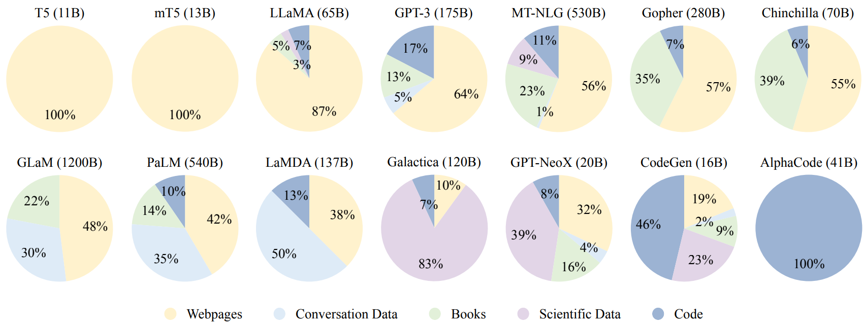
Fig. 11.2 Pretrain data source distribution for existing LLMs. Image from [ZZL+23].

While the scale is one factor impacting resulting model performance (i.e., the scaling law), the quality of data and the ratio of different data types play an equally important role. As dominant pretraining data is from the web, data clearning and quality control is a crucial step for sucessful LLM pretraining [[WLC+19]]. The following Fig. 11.3 summarize the key steps on cleaning training data.

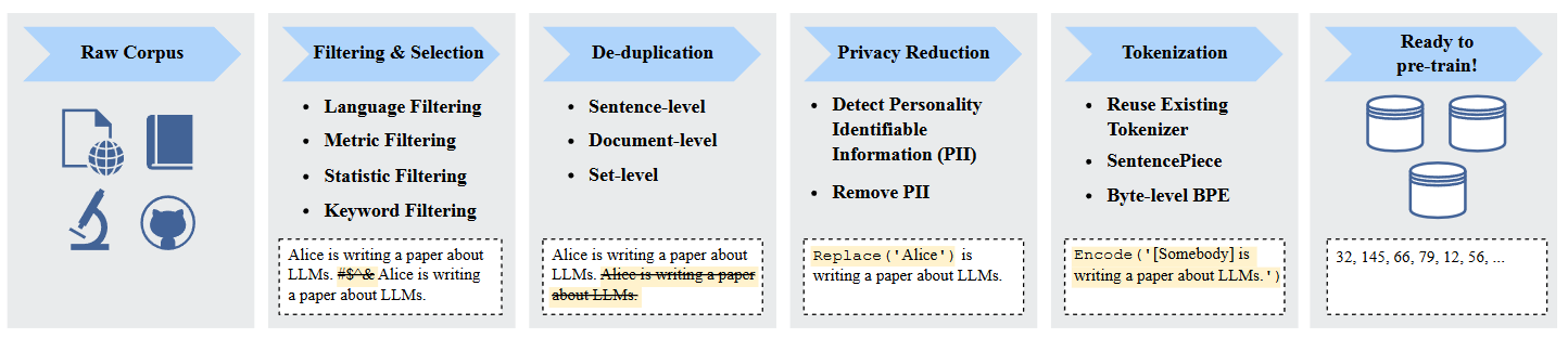
Fig. 11.3 Illustration of data cleaning pipeline for curating LLM pretraining data. Image from [ZZL+23].

Onogoing challenges for constructing LLM pretraining data include:

• Data quality and bias: Ensuring data quality and mitigating biases present in web-scraped data is an ongoing challenge.

• Multilingual representation: Balancing representation across languages, especially for low-resource languages, remains difficult.

11.3.1. Data mixture and schedule

With cleaned data from different data sources, it is essential to design data feeding strategies to pretrain LLM with target capabilities. Two important aspects of data feeding strategy are

• the portition of different data sources

• the order of each data source used in pretraining

11.4. Optimization Algorithms

11.4.1. Minibatch Stochastic Gradient Descent

The classical gradient descent algorithm requires the evaluation of the gradient over the whole set of training data. This is both computational prohibitive and sample inefficient - many samples are similar, making the gradient of the whole data sample is simply the multiplier of the gradient of a much smaller, representative sample data set. Minibatch stochastic gradient descent is much efficient way of gradient descent, which uses a random sample of the training data set to estimate the gradient on each step.

A typical algorithm is showed as follows.

Algorithm 11.1 (Minibatch stochastic gradient descent algorithm)

Inputs Learning rate \(\alpha_k\), iniital model parameter \(\theta\).

Output \(\theta_k\)

1. Set \(k=1\)

2. Repeat until stopping criteria is met:

   1. Sample a minibatch of training samples of size \(m\): \((x^{(i)},y^{(i)}),i=1,2,...,m\).

   2. Compute a gradient estimate over this minibatch samples via

   \[\hat{g}_k = \frac{1}{m}\nabla_{\theta} \sum_{i=1}^{m} L(f(x^{(i)};\theta),y^{(i)}).\]

   3. Apply update \(\theta_k = \theta_k - \alpha_k \hat{g}_k\).

   4. Set \(k=k+1\).

Remark 11.1 (choice of minibatch size)

• The estimation quality of gradient via minibatch gradient descent is strongly affected by the minibatch size. In general, the gradient estimate is unbiased, irrespective of the choice of minibatch size, but its variance will decrease as the minibatch increases.

• For larger minibatch size, we can increase learning rate since the estimated gradient is more certain. There is an empirical Linear Scaling Rule: When the minibatch size is multiplied by \(k\), multiply the learning rate by \(k\) [GDollarG+17].

11.4.2. Adaptive Gradient Method

11.4.2.1. Adaptive Gradient (AdaGrad)

For simple stochastic gradient methods, we need to set the learning rate hyperparameter or even dynamically schedule learning rate, which is usually a difficult task or problem specific. Further, a uniform learning rate is usually not an effective way for high-dimensional gradient descent methods, since one learning rate could be too large for one-dimension but, on the contrary, too small for another dimension.

The AdaGrad algorithm[DHS11] addresses the issue by choosing different learning rates for each dimension. The algorithm adaptively scales the learning rate for each dimension based on the accumulated gradient magnitude on that dimension so far.

Let \(G_k\) be the accumulated gradient up to iteration \(k\), given by

\[G_k = G_{k-1} + \hat{g}_k\odot \hat{g}_k, G_0 = 0.\]

The parameter update is given by

\[\theta_k = \theta_{k-1} - \frac{\alpha_0}{\delta + \sqrt{G_k}} \hat{g}_k\]

where \(\alpha_0\) is the initial learning speed, usually set at a small number (say, 1e-9 to 1e-7) and \(\delta\) is a small positive constant to avoid division by zero.

As we can see, the learning rate in AdaGrad is monotonically decreasing, which may dramatically slow down the convergence as the learning rate becomes too small. In general, AdaGrad algorithm performs best for convex optimization (however, neural network optimization is usually non-convex).

11.4.2.2. RMSProp

As we mentioned before, AdaGrad tend to shrink learning rate too aggressively. This is an advantage when applying AdaGrad to convex function optimization as it enables the algorithm to converge fast and stably. However, non-convex function optimization usually require large, adaptive learning rate to escape bad local minimum and converge stably to better local minimums.

The first remedy is to prevent the learning rate from shrinking too fast. Let \(G_k\) be the accumulated gradient up to iteration \(k\), given by

\[G_k = \rho G_{k-1} + (1- \rho) g_k\odot g_k, G_0 = 0.\]

Then we compute update

\[\theta_k= \theta_{k-1} - \frac{\alpha_0}{\delta + \sqrt{G_k}} \hat{g}_k.\]

which is the core part of the RMSProp algorithm [Hin12].

How this modification can make the \(G_k\) smaller than that in the AdaGrad, as can be seen from following expansion.

Remark 11.2 (Expansion of \(G_k\))

In RMSProp, we have

\[\begin{split} \begin{align} G_k &= \rho G_{k-1} + (1- \rho) g_k\odot g_k \\ &= \rho G_{k-2} + \rho(1- \rho) g_k\odot g_k + \rho(1 - \rho)g_{k-1}\odot g_{k-1} \\ &\approx g\cdot g (1 - \rho) (1 + \rho + \cdot + \rho^{k-1})\\ &= (1 - \rho^k) g\cdot g \end{align} \end{split}\]

where we assume \(g_k\cdot g_k \approx g\cdot g, \forall k\). Clearly, we have roughly,

\[G_k^{RMSProp} \approx \frac{(1 - \rho^k)}{k} G_k^{AdaGrad}, G_k^{AdaGrad}\approx k g\odot g.\]

Remark 11.3 (Importance of adaptive learning rate)

One example to demonstrate the importance of having adaptive learing rate is learning word embeddings. Embeddings of rare words only get limited chances to update because they have limited presence in the training data. On the other hand, embeddings of common words get update frequently. With adaptive learning rate, embeddings of rare words will have large learning rate whenever it gets update. This help the model learn better embeddings for rare words.

11.4.3. Momentum Method

Simple SGD with small learning rate can lead to extremely slow learning for functional surfaces with long, narrow valleys [SMDH13]. One intuition inspired by the physics of a heavy ball falling down is to add momentum to the gradient descent steps. Mathematically, adding momentum is equivalent to adding historical weighted averaged gradient to the current gradient. The total gradient will then be hopefully large enough to enable fast movement on relatively flat regions.

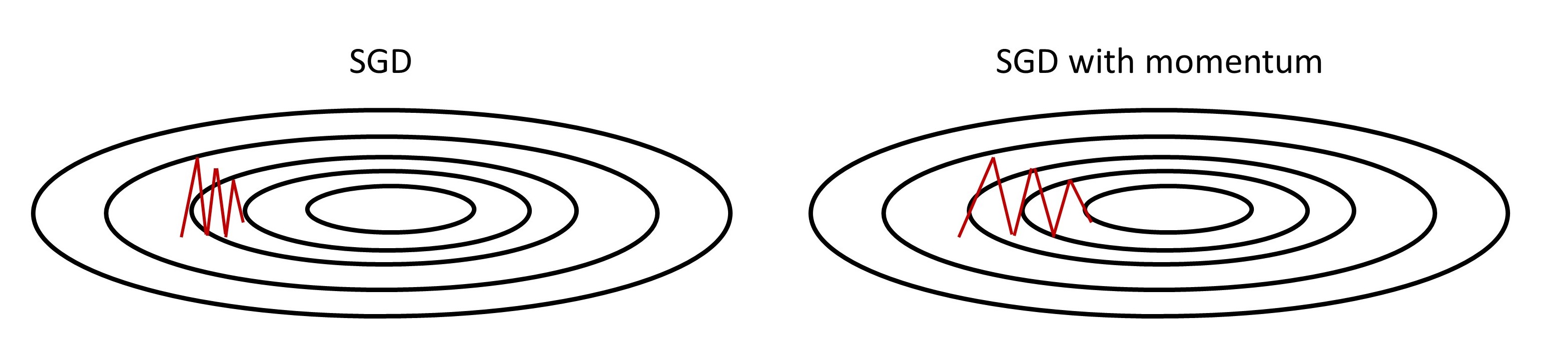
Fig. 11.4 SGD without momentum and with momentum. SGD with momentum can accumulate gradient/velocity in horizontal direction and move faster towards the minimum located at the center.

Consider the gradient

\[\hat{g}_k = \frac{1}{m}\nabla_{\theta} \sum_{i=1}^{m} L(f(x^{(i);\theta}),y^{(i)}),\]

we can compute a speed (an intermedidate parameter) via

\[v_k = \mu v_{k-1} - \alpha_k \hat{g}_k,\]

where \(\mu \in [0, 1]\) is the momentum coefficiency, and \(\alpha_k\) is the learning rate.

The speed (with momentum considered) is then used to update parameter \(\theta\) via

\[\theta_k = \theta_k + v_k.\]

To see that the update velocity is the weighted average gradient, we now show that the velocity is an exponentially decaying moving average (similar to AR(1) process) of the negative gradients, given by

\[\begin{split} \begin{align} v_k &= \alpha v_{k-1} - \hat{g}_k\\ &= \alpha (\alpha v_{k-2} - \hat{g}_{k-1}) - \hat{g}_k \\ &= \alpha^2 v_{k-2} - \alpha \hat{g}_{k-1} - \hat{g}_k \\ &= \cdots \\ &= \sum_{i=0}^\infty \alpha^{i} \hat{g}_{k-i}. \end{align} \end{split}\]

11.4.4. Combined Together: Adam and AdamW

11.4.4.1. Adam

By combining the ideas of momentum and adaptive learning rate, we yield Adam, one of most popular gradient descent algorithm in deep learning community[KB14]. The name Adam is derived from adaptive moment estimation. As its name suggests, Adam will compute velocity via momentum type of averaging and adjust the learning rate using inverse of accumulated gradients.

Specifically, the velocity is computed via

\[\begin{split} \begin{align} M_k &= \rho_1 M_{k-1} + (1-\rho_1)\hat{g}_k \\ \tilde{M}_k &= \frac{M_k}{1-\rho_1^k} \end{align} \end{split}\]

and the accumulated gradient magnitude is compute via

\[\begin{split} \begin{align} G_k &= \rho_2 G_{k-1} + (1-\rho_2)\hat{g}_k \odot \hat{g}_k \\ \tilde{G}_k &= \frac{G_k}{1-\rho_2^k} \end{align} \end{split}\]

Note that we correct the \(M_k\) and \(G_k\) be dividing the factor \(1 - \rho_i^k, i= 1, 2\) to get the average estimation.

The final algorithm is given by the following.

Algorithm 11.2 (Adam stochastic gradient descent algorithm)

Inputs Learning rate \(\alpha\)(set to 0.001), iniital model parameter \(\theta\), decay parameters \(\rho_1\)(set to 0.9), \(\rho_2\)(set to 0.999). \(\delta = 1e-8\)

Output \(\theta_k\)

1. Set \(k=1\).

2. Set \(M_k = 0, G_k = 0\).

3. Repeat until stopping criteria is met：

   1. Sample a minibatch of training samples of size \(m\) \((x^{(i)},y^{(i)}),i=1,2,...,m\).\

   2. compute gradient estimate over minibatch \(N\) samples via

      \[\hat{g}_k = \frac{1}{m}\nabla_{\theta} \sum_{i=1}^{m} L(f(x^{(i);\theta}),y^{(i)}).\]

   3. Accumulate \(M_k = \rho_1 M_{k-1} + (1-\rho_1)\hat{g}_k\). Accumulate \(G_k = \rho_2 G_{k-1} + (1-\rho_2)\hat{g}_k \odot \hat{g}_k\).

   4. Correct biases

      \[\tilde{M}_k = \frac{M_k}{1-\rho_1^k}, \tilde{G}_k = \frac{G_k}{1-\rho_2^k}.\]

   5. Apply update $\(\theta_k = \theta_{k-1} -\frac{\alpha \cdot \tilde{M}_k}{\delta + \sqrt{\tilde{G}_k }}.\)$

   6. Set \(k=k+1\).

11.4.4.2. \(L_2\) Weight Decay and AdamW

\(L_2\) regularization on model parameters often reduce model overfitting and improves the generalization ability of the model. In the SGD optimization framework, the implementation of \(L_2\) regularization term is often realized via weight decay, resulting in an additional term in the gradient that penalize large weights. That is,

\[{g}_{k} \leftarrow \nabla f_{k}\left({\theta}_{k-1}\right)+\lambda {\theta}_{k-1},\]

where \(\lambda\) is the decay parameter, corresponding the strength of the regularization.

AdamW [LH17] is the algorithm that correctly implements Adam with \(L_2\) regularization, which is also called Adam with decoupled weight decay.

The algorithm is given by the following.

Algorithm 11.3 (Adam stochastic gradient descent algorithm with weight decay)

Inputs Learning rate \(\alpha\)(set to 0.001), iniital model parameter \(\theta\), decay parameters \(\rho_1\)(set to 0.9), \(\rho_2\)(set to 0.999). \(\delta = 1e-8\). Weight decay parameter \(\lambda \in \mathbb{R}\).

Output \(\theta_k\)

1. Set \(k=1\).

2. Set \(M_k = 0, G_k = 0\).

3. Repeat until stopping criteria is met：

   1. Sample a minibatch of training samples of size \(m\) \((x^{(i)},y^{(i)}),i=1,2,...,m\).\

   2. compute gradient estimate over minibatch \(N\) samples via

      \[\hat{g}_k = \frac{1}{m}\nabla_{\theta} \sum_{i=1}^{m} L(f(x^{(i);\theta}),y^{(i)}).\]

   3. Accumulate \(M_k = \rho_1 M_{k-1} + (1-\rho_1)\hat{g}_k\). Accumulate \(G_k = \rho_2 G_{k-1} + (1-\rho_2)\hat{g}_k \odot \hat{g}_k\).

   4. Correct biases

      \[\tilde{M}_k = \frac{M_k}{1-\rho_1^k}, \tilde{G}_k = \frac{G_k}{1-\rho_2^k}.\]

   5. Apply update

   \[\theta_k = \theta_{k-1} -\frac{\alpha \cdot \tilde{M}_k}{\delta + \sqrt{\tilde{G}_k }} - \lambda \theta_{k}.\]
   6. Set $k=k+1$.

11.5. Bibliography

[BJT+22]

Mohammad Bavarian, Heewoo Jun, Nikolas Tezak, John Schulman, Christine McLeavey, Jerry Tworek, and Mark Chen. Efficient training of language models to fill in the middle. arXiv preprint arXiv:2207.14255, 2022.

[CTJ+21]

Mark Chen, Jerry Tworek, Heewoo Jun, Qiming Yuan, Henrique Ponde De Oliveira Pinto, Jared Kaplan, Harri Edwards, Yuri Burda, Nicholas Joseph, Greg Brockman, and others. Evaluating large language models trained on code. arXiv preprint arXiv:2107.03374, 2021.

[DALF+24]

DeepSeek-AI, Aixin Liu, Bei Feng, Bing Xue, Bingxuan Wang, and others. Deepseek-v3 technical report. 2024. URL: https://arxiv.org/abs/2412.19437, arXiv:2412.19437.

[DHS11]

John Duchi, Elad Hazan, and Yoram Singer. Adaptive subgradient methods for online learning and stochastic optimization. Journal of Machine Learning Research, 12(Jul):2121–2159, 2011.

[GIRoziere+24] (1,2)

Fabian Gloeckle, Badr Youbi Idrissi, Baptiste Rozière, David Lopez-Paz, and Gabriel Synnaeve. Better & faster large language models via multi-token prediction. arXiv preprint arXiv:2404.19737, 2024.

[GDollarG+17]

Priya Goyal, Piotr Dollár, Ross Girshick, Pieter Noordhuis, Lukasz Wesolowski, Aapo Kyrola, Andrew Tulloch, Yangqing Jia, and Kaiming He. Accurate, large minibatch sgd: training imagenet in 1 hour. arXiv preprint arXiv:1706.02677, 2017.

[GZY+24]

Daya Guo, Qihao Zhu, Dejian Yang, Zhenda Xie, Kai Dong, Wentao Zhang, Guanting Chen, Xiao Bi, Yu Wu, YK Li, and others. Deepseek-coder: when the large language model meets programming–the rise of code intelligence. arXiv preprint arXiv:2401.14196, 2024.

[HKK+20]

Tom Henighan, Jared Kaplan, Mor Katz, Mark Chen, Christopher Hesse, Jacob Jackson, Heewoo Jun, Tom B Brown, Prafulla Dhariwal, Scott Gray, and others. Scaling laws for autoregressive generative modeling. arXiv preprint arXiv:2010.14701, 2020.

[Hin12]

Geoffrey Hinton. Neural Networks for Machine Learning. University of Toronto, 2012.

[KMH+20]

Jared Kaplan, Sam McCandlish, Tom Henighan, Tom B Brown, Benjamin Chess, Rewon Child, Scott Gray, Alec Radford, Jeffrey Wu, and Dario Amodei. Scaling laws for neural language models. arXiv preprint arXiv:2001.08361, 2020.

[KB14]

Diederik P Kingma and Jimmy Ba. Adam: a method for stochastic optimization. arXiv preprint arXiv:1412.6980, 2014.

[LAZ+23]

Raymond Li, Loubna Ben Allal, Yangtian Zi, Niklas Muennighoff, Denis Kocetkov, Chenghao Mou, Marc Marone, Christopher Akiki, Jia Li, Jenny Chim, and others. Starcoder: may the source be with you! arXiv preprint arXiv:2305.06161, 2023.

[LH17]

Ilya Loshchilov and Frank Hutter. Decoupled weight decay regularization. arXiv preprint arXiv:1711.05101, 2017.

[SMDH13]

Ilya Sutskever, James Martens, George Dahl, and Geoffrey Hinton. On the importance of initialization and momentum in deep learning. In International conference on machine learning, 1139–1147. 2013.

[WLC+19]

Guillaume Wenzek, Marie-Anne Lachaux, Alexis Conneau, Vishrav Chaudhary, Francisco Guzmán, Armand Joulin, and Edouard Grave. Ccnet: extracting high quality monolingual datasets from web crawl data. arXiv preprint arXiv:1911.00359, 2019.

[ZZL+23] (1,2)

Wayne Xin Zhao, Kun Zhou, Junyi Li, Tianyi Tang, Xiaolei Wang, Yupeng Hou, Yingqian Min, Beichen Zhang, Junjie Zhang, Zican Dong, Yifan Du, Chen Yang, Yushuo Chen, Zhipeng Chen, Jinhao Jiang, Ruiyang Ren, Yifan Li, Xinyu Tang, Zikang Liu, Peiyu Liu, Jian-Yun Nie, and Ji-Rong Wen. A survey of large language models. arXiv preprint arXiv:2303.18223, 2023.