16. *Reinforcement Learning Essentials

16.1. Reinforcement learning framework

16.1.1. Notations

• \(S_t, s_t\) :state at time \(t\); \(S_t\) denotes random variable; \(s_t \) denotes one realization.

• \(A_t, a_t\) :action at time \(t\); \(A_t\) denotes random variable; \(a_t \) denotes one realization.

• \(R_t\) :reward at time \(t\).

• \(\gamma\) :discount rate (\(0 \leq \gamma \leq 1\)).

• \(G_t\) :discounted return at time \(t\) (\(\sum_{k=0}^\infty \gamma^k R_{t+k+1}\)).

• \(\mathcal{S}\) :set of all states, also known as state space.

• \(\mathcal{S}^T\) :set of all terminal states.

• \(\mathcal{A}\) :set of all actions, also known as action space .

• \(\mathcal{A}(s)\) :set of all actions available in state \(s\).

• \(p(s'|s,a)\) :transition probability to reach next state \(s'\), given current state \(s\) and current action \(a\).

• \(\pi, \mu\) :policy.

  • if deterministic: \(\pi(s) \in \mathcal{A}(s)\) for all \(s \in \mathcal{S}\).

  • if stochastic: \(\pi(a|s) = \mathbb{P}(A_t=a|S_t=s)\) for all \(s \in \mathcal{S}\) and \(a \in \mathcal{A}(s)\).

• \(V^\pi\) :state-value function for policy \(\pi\) (\(v_\pi(s) \doteq E[G_t|S_t=s]\) for all \(s\in\mathcal{S}\)).

• \(Q^\pi\) :action-value function for policy \(\pi\) (\(q_\pi(s,a) \doteq E[G_t|S_t=s, A_t=a]\) for all \(s \in \mathcal{S}\) and \(a \in \mathcal{A}(s)\)).

• \(V^*\) :optimal state-value function (\(v_*(s) \doteq \max_\pi V^\pi(s)\) for all \(s \in \mathcal{S}\)).

• \(Q^*\) :optimal action-value function (\(q_*(s,a) \doteq \max_\pi Q^\pi(s,a)\) for all \(s \in \mathcal{S}\) and \(a \in \mathcal{A}(s)\)).

16.1.2. Overview

In essence, we can view reinforcement learning (RL) as a data-driven way to solve the policy optimization problem in a MDP (Markov Decision Process). In RL, we use a setting that contains an agent and an environment [Fig. 16.1], where data are collected through agent-environment interactions and then further utilized to optimize policies. The agent iteratively takes action specified by a policy, interacts with the environment, and ultimately learn ‘knowledge or strategies’ from the interactions. At every step, the agent makes an observation of the environment (we called a state or an observation), then it chooses an action to take. The environment will respond to the agent’s action by changing its state and providing a reward signal to the agent, which serves as a gauge on the quality of the agent’s current action. The goal of the agent, however, is not to maximize the immediate reward of an action, but is to maximize its cumulative reward along the whole process.

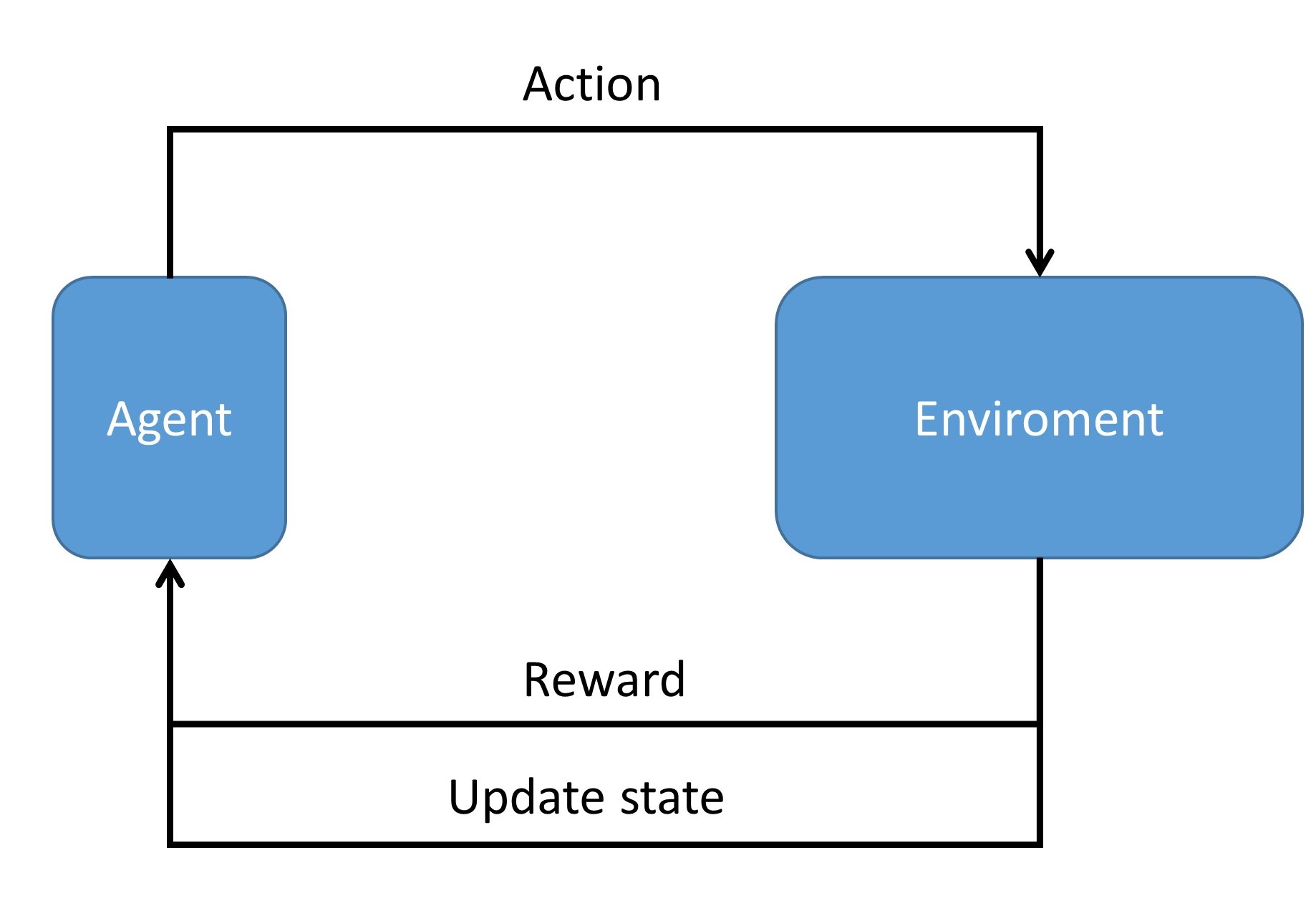
Fig. 16.1 One core component in reinforcement learning is agent environment interaction. The agent takes actions based on observations on the environment and a decision-making module that maps observations to action. The environment model updates system state and provides rewards according to the action

For example, in the Atari game Breakout [Fig. 16.2], we assume an agent controls the bat to deflect the ball to destroy the bricks. The actions allowed are moving left and moving right; the state includes positions of the ball, the bat, and all the bricks; rewards will be given to the agent if bricks are hit. The environment, represented by a physical simulator, will simulate the ball’s trajectory and collision between the ball and the bricks. The ultimate goal is learn a control policy that specifies the action to take after observing a state.

Fig. 16.2 Scheme of the Atari game breakout.

In finite state MDP, we introduce the two step iterative framework consisting of policy evaluation and policy improvement to seek optimal control policies. Although the agent-environment interaction paradigm seems to be vastly different from the Markov decision framework, many reinforcement learning algorithms can also be interpreted under this two step framework. We can view the agent-environment interaction process under a specified policy as policy evaluation step based on the rewards received from the environment. With the estimated value functions, we can similarly apply the policy improvement methods [Fig. 16.3].

The sharp contrast between MDP and reinforcement learning is that reinforcement learning is model-free learning, the knowledge of the environment is from agent-environment interaction data. On the other hand, MDP is model-based learning, meaning that the agent already know beforehand all the responses and rewards from environment for every action it takes. For complex read-world problems where models are not available, reinforcement learning offers a viable approach to learning optimal control policy via gradually building up the knowledge of the environment.

How much knowledge of the environment should the agent gain before the agent starts to improve the policy? Exploring the environment sufficiently would be prohibitive; on the other hand, improving the policy based on limited knowledge can produce inferior policies. The balance of environment exploration and policy improvement is known as the exploration-exploitation dilemma. One common way out is the \(\epsilon\) greedy action selection, where the agent has \((1-\epsilon)\) probability to continue to collect more samples based on currently perceived optimal control policy to improve current policy and \(\epsilon\) probability to randomly explore the environment via random actions.

Fig. 16.3 Policy evaluation and policy improvement framework in the context reinforcement learning.

16.1.3. Finite-state MDP

Definition 16.1 (Finite state Markov decision process (MDP))

A finite state Markov decision process (MDP) is characterized by a tuple \((\mathcal{S}, \mathcal{A}, \mathcal{P})\) where \(\mathcal{S}\) is the state space, \(\mathcal{A}\) is the action space, and \(\mathcal{P} = \{p(s'|s, a), s,s'\in \mathcal{S}, a\in \mathcal{A}\}\) is the state transition probability. We require \(\mathcal{S}, \mathcal{A}\) to have finite number of elements.
The goal is compute an optimal control policy \(\pi^*: \mathcal{S}\to \mathcal{A}\) such that the expected total reward in the process

\[ J = E[\sum_{t=0}^\infty \gamma^t R(s_{t+1}, a_t)] \]

is maximized, where \(R(s,a):\mathcal{S}\times\mathcal{A}\to{\mathbb(R)}\) is the one-step reward function and \(\gamma \in [0, 1)\) is the discount factor.

Example 16.1 (examples of reward functions)

• In a navigation task, we can set \(r(s_t,a_t) = \mathbb{I}(s_t \in S_{target})\).

• In a game, the state of gaining scores has a reward 1 and other states have a reward 0.

Definition 16.2 (value functions)

• Let \(\pi\) be a given control policy. We can define a value function associated with this policy by

  \[V^\pi(s) = E^\pi[\sum_{t=0}^\infty \gamma^t R(s_{t+1}, a_t)|s_0 = s, \pi],\]

  which is the expected total rewards by following a given policy \(\pi\) starting from initial state \(s\).

• Given a value function associated with a policy \(\pi\), we can obtain \(\pi\) via

  \[\pi(s) = \max_{a\in\mathcal{A}(s)}\sum_{s' \in \mathcal{S}}p(s'|s,a)(r + \gamma V(s'))\]

  where \(r = R(s', a)\) is the reward received at state \(s'\) after taking action \(a\) at \(s\).

• The optimal value function \(V^*\) and the optimal policy \(\pi^*\) are connected via

  \[V^*(s) = \max_{\pi} V^\pi(s), \pi^*(s) = \max_{\pi} V^\pi(s).\]

Lemma 16.1 (recursive relationship of value functions)

Given a value function \(V^\pi\) associated with a control policy \(\pi\). The value function satisfies the following backward relationship:

\[V^\pi(s) = E_{s'\sim P(s'|s, a = \pi(s))}[R(s',a)+ \gamma V^\pi(s')].\]

Particularly, we have the Bellman’s equation characterizing the optimal value function by

\[V^*(s) = \max_aE_{s'\sim P(s'|s, a )}[R(s',a)+ \gamma V^*(s')].\]

Proof. The definition of \(V^\pi\) says

\[\begin{split}\begin{align*} V^\pi(s) &= E^\pi[\sum_{t=0}^\infty \gamma^t R(s_{t+1}, a_t)|s_0 = s, \pi]\\ &=E_{s_1\sim P(s_1|s_0, a = \pi(s))} [R(s_{1}, a_0) + E^\pi[\sum_{t=1}^\infty \gamma^t R(s_{t+1}, a_t)|s_1 = s', \pi]|s_0 = s, \pi]\\ &=E_{s_1\sim P(s_1|s_0, a = \pi(s))} [R(s_{1}, a_0) + V(s_1)|s_0 = s, \pi] \end{align*}\end{split}\]

where we have used the tower property of conditional expectation.

16.1.4. State-action Value function (\(Q\) function)

Like value function in a finite state MDP, \(Q\) functions [] play the same critical role in reinforcement learning. Now we go through their formal definition and their recursive relations.

Definition 16.3 (state-action value function - \(Q\) function)

• The state-action value function \(Q^\pi:S\times A\to \mathbb(R)\) associated with a policy \(\pi\) is defined as the expected return starting from state \(s\), taking action \(a\) and thereafter following the policy \(\pi\), given as

  \[Q^\pi(s,a) = E^\pi \{\sum_{t=0}^\infty \gamma^t R(s_{t+1}, a_t)|s_0 = s,a_t = a\}.\]

• The optimal state-action value function \(Q^*:S\times A\to \mathbb(R)\) is defined as the expected return starting from state \(s\), taking action \(a\) and thereafter following an optimal policy \(\pi^*\), such that

  \[Q^*(s,a) = \max_{\pi} Q^\pi(s,a) \]

• The optimal policy \(\pi^*\) is related to \(Q^*\) as

  \[\pi^*(s) = \arg \max_a Q^*(s,a).\]

• The value function associated with a policy \(\pi\),

  \[V^\pi(s) = E^\pi \{\sum_{t=0}^\infty \gamma^t R(s_{t+1}, a_t)|s_0 = s\}.\]

• The value function \(V(s)\) is connected with \(Q(s,a)\) via

  \[V^\pi(s) = Q(s, \pi(s)).\]

• The optimal state-action value function is connected to value function via

  \[V^*(s) = \max_{a} Q^*(s,a).\]

Lemma 16.2 (recursive relations of the Q function)

• The state-action value function will satisfy

\[\begin{split}\begin{align*} Q^\pi(s,a) &= E^\pi_{s'\sim p(s'|s,\pi(s))} [R(s', a) + \gamma Q^\pi(s',\pi(s'))] \\ &=E^\pi_{s'\sim p(s'|s,\pi(s))} [R(s',a) + \gamma V^\pi(s')], \end{align*}\end{split}\]

where the expectation is taken with respect to the distribution of \(s'\)(the state after taking \(a\) at \(s\)) and we use the definition \(V^\pi(s') = Q^\pi(s',\pi(s'))\).

• Particularly, the optimal state-action value function will satisfy

\[\begin{split}\begin{align*} Q^*(s,a) &= E^{\pi^*}_{s'\sim p(s'|s,\pi^*(s))}[R(s',a) + \gamma \max_{a\in A(s')} Q*(s',a)]\\ &= E^{\pi^*}_{s'\sim p(s'|s,\pi^*(s))}[R(s',a) + \gamma V^*(s')] \end{align*}\end{split}\]

where the expectation is taken with respect to the distribution of \(s'\)(the state after taking \(a\) at \(s\)) we use the definition \(V^*(s') = \max_a Q^*(s',a) = Q^*(s',\pi^*(s'))\).

Proof. (1) From the definition \(Q^\pi(s, a)\), we have

\[\begin{split}\begin{align*} Q^\pi(s,a) &= E^\pi [\sum_{t=0}^\infty \gamma^t r_{t+1}|s_0 = s,a_t = a] \\ &= E^\pi [r_{1} + \sum_{k=1}^\infty \gamma^k r_{t+1}|s_0 = s,a_t = a] \\ &= E^\pi [r_{1} + E^{\pi}[\sum_{k=1}^\infty \gamma^k r_{t+1}|s_1 = s, a_1 = \pi(s_1)]|s_0 = s,a_t = a] \\ &= E^\pi [r_{1}|s_0 = s,a_t = a\} + Q^\pi(s_1,\pi(s_1))|s_0 = s,a_t = a] \end{align*}\end{split}\]

where we have used the tower property of conditional expectation.

(2) From (1) we have

\[Q^*(s,a) = {E}^*_{s'\sim p(s'|s,\pi(s))} [r + \gamma Q^*(s',\pi^*(s'))].\]

Further note that \(\pi^*(s') = \arg\max_{a\in \mathcal(A)(s')} Q(s',a')\)

Remark 16.1 (recursive relation for value functions)

Recall that in Lemma 16.1, we have covered the recursive relation for value functions.

• Given a value function \(V^\pi\) associated with control policy \(\pi\). The value function satisfies the following backward relationship:

  \[V^\pi(s) = E_{s'\sim P(s'|s, a = \pi(s))}[R(s',a)+ \gamma V^\pi(s')].\]

• Particularly, we have the Bellman’s equation saying that

• \[V^*(s) = \max_aE_{s'\sim P(s'|s, a ))}[R(s',a)+ \gamma V^*(s')].\]

Note that in above two cases, \(a\) is determined by either the policy function \(\pi\) or the maximization. \(a\) is not a free variable.

16.1.5. Policy iteration and Value iteration

16.1.5.1. Policy iteration

The core idaa underlying policy iteration is to iteratively carry out two procedures: policy evaluation and policy improvement [Fig. 16.4]. Given a starting policy \(\pi\), we perform policy evaluation to estimate the value function \(V^\pi\) associated with this policy; then we improve the policy via dynamic programming principles, or the Bellman Principle.

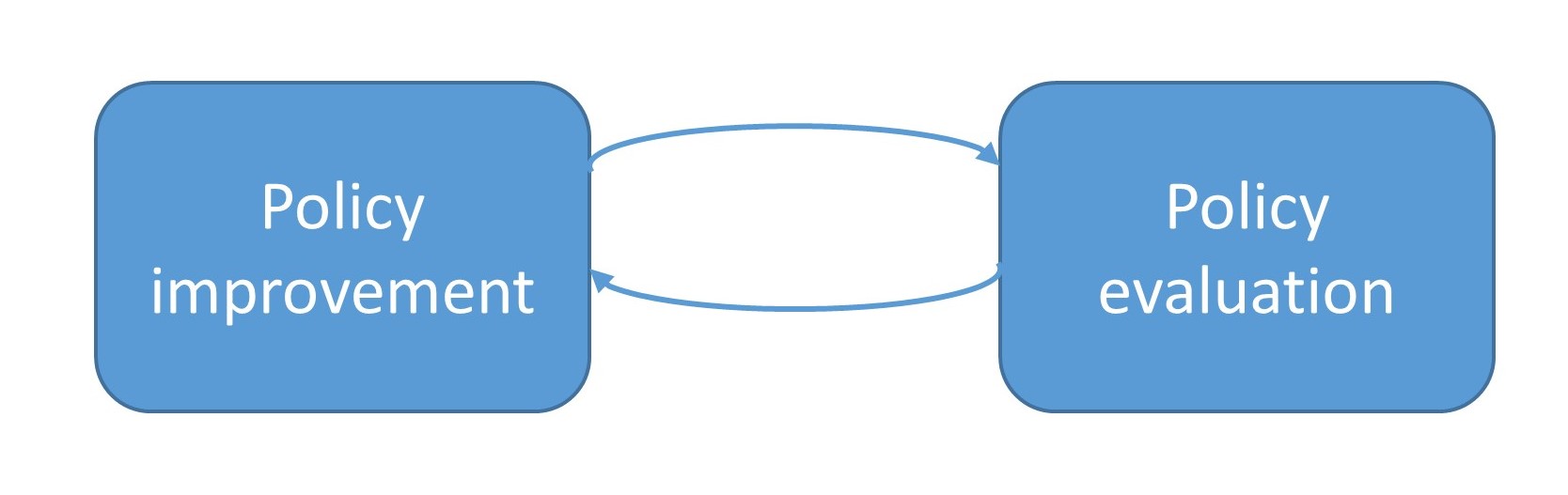
Fig. 16.4 Policy iteration involves iteratively carrying out policy evaluation and policy improvement procedures.

The policy evaluation step involves estimating value function \(V^\pi\) given a policy \(\pi\). We can use the following iterative steps:

\[V^{k+1}(s) = \sum_{s' \in \mathcal{S}}p(s'|s,a = \pi(s))(r + \gamma V^{k}(s')), \forall s\in \mathcal{S}.\]

where superscript \(k\) is the iteration index.

\(V^{k}(s)\) will converge to value function \(V^\pi\), as we show in the following [Theorem 16.1].

Theorem 16.1 (convergence property of iterative policy evaluation)

For a finite state MDP, we can write the value function recursive relationship explicitly as

\[V^\pi(s) = \sum_{s'\in \mathcal{S}}P(s'|s, a = \pi(s))[R(s',a)+ \gamma V^\pi(s')].\]

We can express the recursive relationship as a matrix form given by

\[V = T(R + \gamma V),\]

where \(R,V \in \mathbb(R)^{|\mathcal{S}|}, T\in \mathbb(R)^{|\mathcal{S}|\times |\mathcal{S}|}\).

We further define \(H(V) \triangleq T(R + \gamma V)\) as the policy evaluation operator.

We have

• \(H\) is a contraction mapping.

• In iterative policy evaluation, \(V^{k}(s)\) will converge to value function \(V^\pi\). Or equivalently, \(V^\pi\) is the fixed point of \(H\), and

\[\lim_{n\to\infty} H^{n}(V) = V^\pi.\]

• (error bound) If \(\lVert H^k(V) - H^{k-1 \rVert(V)}_\infty \leq \epsilon,\) then

\[\lVert {H^k(V) - V^\pi} \rVert_\infty \leq \frac{\epsilon}{1 - \gamma}.\]

Proof. (1)

\[\begin{split}\begin{align*} \begin{array}{l}{\|H(\tilde{V})-H(V)\|_{\infty}} \\ {=\| TR+\gamma T \tilde{V}-TR-\gamma T V||_{\infty} \text { (by definition) }} \\ {=|| \gamma T(\tilde{V}-V)||_{\infty} \quad \text { (simplification) }} \\ {\left.\leq \gamma|| T||_{\infty}|| \tilde{V}-V||_{\infty} \quad \text { (since }\|A B\| \leq\|A\|\|B\|\right)} \\ {\left.=\gamma|| \tilde{V}-V||_{\infty} \quad \text { (since } \max _{s} \sum_{s^{\prime}} T\left(s, s^{\prime}\right)=1\right)}\end{array} \end{align*}\end{split}\]

(2) Note that from Fixed point Theorem, we have

\[\lVert H^{n \rVert(V) - V^\pi}_\infty \leq \gamma^n \lVert V - V^\pi \rVert_\infty.\]

Therefore,

\[\lim_{n\to\infty} H^{n}(V) = V^\pi.\]

Remark 16.2 (error estimation and stopping criterion)

The third property can be used as a stopping criterion during iterations. Suppose the tolerance is \(Tol\), then we should iterate until the maximum change during consecutive iteration is small than \((1 - \gamma)\times Tol\).

Given a learned value function \(V^\pi\) of a policy \(\pi\), we can derive its \(Q\) function counterpart via

\[Q(s,a) = \sum_{s' \in \mathcal{S}}p(s'|s,a)(R(s',a)+\gamma V^\pi(s')), \forall s, a.\]

\(Q\) function offer a convenient way to improve current policy \(\pi\). Indeed, by relying on following policy improvement theorem [], we can consistently improve our policy towards the optimal one.

Theorem 16.2 (policy improvement theorem)

Define the \(Q\) function associated with a policy \(\pi\) as

\[Q^\pi(s,a) = \sum_{s' \in \mathcal{S}}p(s'|s,a)(R(s',a)+\gamma V^\pi(s')), \forall s, a.\]

Let \(\pi\) and \(\pi'\) be two policies. If \(\forall s\in \mathcal(S)\),

\[Q^\pi(s, \pi'(s)) \geq V^\pi(s),\]

then

\[V^{\pi'}(s) \geq V^\pi(s), \forall s\in \mathcal(S).\]

That is \(\pi'\) is a better policy than \(\pi\).

Based on this theorem, we can create a better policy via following greedy manner (known as policy improvement procedure)

\[\pi'(s) = \arg\max_{a\in\mathcal{A}(s)}Q(s,a), \forall s.\]

Given a value function \(V\), we can improve the policy implicitly associated with the value function via two steps:

• First calculate the intermediate \(Q\) function

\[Q(s,a) = \sum_{s' \in \mathcal{S}}p(s'|s,a)(r+\gamma V(s')), \forall s, a.\]

• Second improve the policy by $\(\pi'(s) = \arg\max_{a\in\mathcal{A}(s)}Q(s,a), \forall s.\)$

Notably, let \(\pi'\) be the improved greedy policy, if \(V^{\pi'} = V^\pi\), then \(\pi\) is the optimal policy, based on the definition and recursive relation of \(V\) [Lemma 16.1].

The following algorithm summarizes the policy iteration method [].

Algorithm 16.1 (The policy iteration algorithm for MDP)

Inputs MDP model, a small positive number \(\tau\).

Output Policy \(\pi \approx \pi^*\)

1. Initialize \(\pi\) arbitrarily (e.g., \(\pi(a|s)=\frac{1}{|\mathcal{A}(s)|}\) for all \(s \in \mathcal{S}\) and \(a \in \mathcal{A}(s)\))

2. Set policyStable = false

3. Repeat until policy_table = true:

   1. \(V \leftarrow \text{Policy_Evaluation}(\text{MDP}, \pi, \tau)\).

   2. \(\pi' \leftarrow \text{Policy_Improvement}(\text{MDP}, V)\)

   3. If{\(\pi= \pi'\)} policyStable = true$

   4. \(\pi = \pi'\)

16.1.5.2. Value iteration

The policy iteration method iterates the two steps of evaluating policy and improving policy. Alternatively, we can also directly iteratively estimate the optimal value function, the value function associated the optimal policy, without evaluating the policy associated with value functions. In fact, since policies can be directly calculated from a given value function, having the optimal value function will just give us the optimal policy.

Let \(V^{(0)}\) be an initial value function. Based on the value iteration theorem [Theorem 16.3], we can design iteration like

\[V^{(k+1)}(s) = \max_a\sum_{s'\in \mathcal{S}}P(s'|s, a )[R(s',a)+ \gamma V^{(k)}(s')], \forall s\in \mathcal{S}.\]

where \(k\) is the iteration number. The following theorem shows that this iteration procedure will lead to convergence to the optimal value function.

More formally, we have

Theorem 16.3 (convergence property of value iteration)

For a finite state MDP, we can write the optimal value function recursive relationship as

\[V^*(s) = \max_a\sum_{s'\in \mathcal{S}}P(s'|s, a )[R(s',a)+ \gamma V^*(s')], \forall s\in \mathcal{S}.\]

We can express the recursive relationship as a matrix form given by

\[V = T(R + \gamma V),\]

where \(R,V \in \mathbb(R)^{|\mathcal{S}|}, T\in \mathbb(R)^{|\mathcal{S}|\times |\mathcal{S}|}\).

We further define \(H(V) \triangleq \max_a T(R + \gamma V)\) as the value iteration operator.

We have

• \(H\) is a contraction mapping.

• In iterative policy evaluation, \(V^{k}(s)\) will converge to the unique optimal value function \(V^*\). Or equivalently, \(V^*\) is the fixed point of the contraction mapping \(H\), and $\(\lim_{n\to\infty} H^{n}(V) = V^*.\)$

• (error bound) If \(\lVert H^k(V) - H^{k-1 \rVert(V)}_\infty \leq \epsilon,\) then \(\lVert H^k(V) - V^* \rVert_\infty \leq \frac{\epsilon}{1 - \gamma}.\)

A direct application of the value iteration theorem gives the following value iteration algorithm [Algorithm 16.2].

\begin{algorithm}[H] \KwIn{MDP, small positive number \(\epsilon\) as tolerance } \KwOut{Value function \(V \approx V^*\) and policy \(\pi \approx \pi^*\). } Initialize \(V\) arbitrarily. Set (\(V(s)=0\) for all \(s \in \mathcal{S}^T\).)\ \mathbb(R)epeat{\(\Delta < \epsilon\)}{ \(\Delta = 0\)\ \For{\(s \in \mathcal{S}\)}{ \(v = V(s)\)\ \(V(s) = \max_{a\in\mathcal{A}(s)}\sum_{s' \in \mathcal{S}}P(s'|s,a)(R(s',a) + \gamma V(s'))\)\ \(\Delta = \max(\Delta, |v-V(s)|)\) } } Compute the policy \(\pi(s) = \max_{a\in\mathcal{A}(s)}\sum_{s' \in \mathcal{S}}P(s'|s,a)(R(s',a) + \gamma V(s'))\). \ \KwRet{\(V\) and \(\pi\)} \caption{Value iteration algorithm for a finite state MDP}\label{ch:reinforcement-learning:alg:valueIterationAlg} \end{algorithm}

Algorithm 16.2 (Value iteration algorithm for a finite state MDP)

Inputs MDP, a small positive number \(\tau\) as tolerance

Output Value function \(V \approx V^*\) and policy \(\pi \approx \pi^*\).

1. Initialize \(V\) arbitrarily. Set (\(V(s)=0\) for all \(s \in \mathcal{S}^T\).)

2. Set policyStable = false

3. Repeat until \(\Delta < \tau\):

   1. \(\Delta = 0\). For \(s \in \mathcal{S}\):

      1. \(v = V(s)\)

      2. \(V(s) = \max_{a\in\mathcal{A}(s)}\sum_{s' \in \mathcal{S}}P(s'|s,a)(R(s',a) + \gamma V(s'))\)

      3. \(\Delta = \max(\Delta, |v-V(s)|)\)

4. Compute the policy

   \[\pi(s) = \max_{a\in\mathcal{A}(s)}\sum_{s' \in \mathcal{S}}P(s'|s,a)(R(s',a) + \gamma V(s')).\]

Remark 16.3 (value iteration vs. policy iteration; model-based vs. model-free)

• At the first glance, it may seem the simplicity of the value iteration method will make the policy iteration method obsolete. It is critical to know that value iteration requires the knowledge of model, which is represented by the transition probabilities \(p(s'|s, a)\).

• Later we will see that for many complicated real-world decision-making problems, a model is a luxury and often unavailable. In such situations, we usually turn to reinforcement learning, a model-free, data-driven approach to learn control policies. Most reinforcement learning algorithms, from a high-level abstraction, are comprised of the two steps of policy evaluation and policy improvement.