23. Text Embedding Fundamentals

23.1. Introduction

There are many NLP tasks involves determining the relationship of two sentences, including semantic similarity, semantic relation reasoning, questioning answering etc. For example, Quora needs to determine if a question asked by a user has a semantically similar duplicate. The GLUE benchmark as an example [\autoref{ch:neural-network-and-deep-learning:ApplicationNLP:sec:BERTDownstreamTasks}], 6 of them are tasks that require learning sentences Inter-relationship. Specifically,

MRPC: The Microsoft Research Paraphrase Corpus [DB05] is a corpus of sentence pairs automatically extracted from online news sources, with human annotations for whether the sentences in the pair are semantically equivalent.

QQP: The Quora Question Pairs dataset is a collection of question pairs from the community question-answering website Quora. The task is to determine whether a pair of questions are semantically equivalent. As in MRPC, the class distribution in \(\mathrm{QQP}\) is unbalanced \((63 \%\) negative), so we report both accuracy and F1 score. We use the standard test set, for which we obtained private labels from the authors. We observe that the test set has a different label distribution than the training set.

STS-B: The Semantic Textual Similarity Benchmark [CDA+17] is a collection of sentence pairs drawn from news headlines, video and image captions, and natural language inference data.

Natural language inference: [BAPM15] Understanding entailment and contradiction is fundamental to understanding natural language, and inference about entailment and contradiction is a valuable testing ground for the development of semantic representations. The semantic concepts of entailment and contradiction are central to all aspects of natural language meaning, from the lexicon to the content of entire texts. Natural language inference is the task of determining whether a hypothesis is true (entailment), false (contradiction), or undetermined (neutral) given a premise.

Table 23.1 Entailment, contradiction, and neural examples in a natural language inference task.

Premise	Label	Hypothesis
A man inspects the uniform of a figure in some East Asian country.	Contraction	The man is sleeping.
An older and younger man smiling.	Neutral	Two men are smiling and laughing at the cats playing on the floor.
A soccer game with multiple males playing.	Entailment	Some men are playing a sport.

Although BERT model and its variant have achieved new state-of-the-art among many sentence-pair classification and regression tasks. It has many practical challenges in tasks like large-scale semantic similarity comparison, clustering, and information retrieval via semantic search, etc. These tasks require that both sentences are fed into the network, which causes a massive computational overhead for large BERT model. Considering the task of finding the most similar pair among \(N\) sentences, then it requires \(N^2/2\) forward pass computation of BERT.

An alternative approach is to derive a semantically meaningful sentence embeddings for each sentence. A sentence embedding is a dense vector representation of a sentence. Sentences with similar semantic meanings are close and sentences with different meanings are apart. With sentence embeddings, similarity search can be realized simply via a distance or similarity metrics, such as cosine similarity. Besides performing similarity comparison between two sentences, the sentence embedding can also be used as generic sentence feature for different NLP tasks.

Early on, there have been efforts directed to derive sentence embedding by aggregating word embeddings. For example, one can average the BERT token embedding output as the sentence embedding. Another common practice is to use the output of the first token (the [CLS] token) as the sentence, which is found to be worse than averaging GloVe embeddings\cite{reimers2019sentence}. Recently, contrastive learning and Siamese type of learning have been successfully applied in deriving sentence embeddings, which will be the focus of our following sections.

Remark 23.1 (Why we need sentence embedding fine tuning)

Pre-trained BERT models do not produce efficient and independent sentence embeddings as they always need to be fine-tuned in an end-to-end supervised setting. This is because we can think of a pre-trained BERT model as an indivisible whole and semantics is spread across all layers, not just the final layer. Without fine-tuning, it may be ineffective to use its internal representations independently. It is also hard to handle unsupervised tasks such as clustering, topic modeling, information retrieval, or semantic search. Because we have to evaluate many sentence pairs during clustering tasks, for instance, this causes massive computational overhead.

23.2. Contextual Text Embedding Fundamentals

23.2.1. Anisotropy

[Eth19]

Contextualized representations are anisotropic in all non-input layers. If word representations from a particular layer were isotropic (i.e., directionally uniform), then the average cosine similarity between uniformly randomly sampled words would be 0. The closer this average is to 1, the more anisotropic the representations. The geometric interpretation of anisotropy is that the word representations all occupy a narrow cone in the vector space rather than being uniform in all directions; the greater the anisotropy, the narrower this cone.

As seen in Fig. 23.1, this implies that in almost all layers of BERT and GPT-2, the representations of all words occupy a narrow cone in the vector space.

Contextual word embeddings are generally more anisotropic in higher layers.

anisotropy is also viewed as representation degeneration problem [GHT+19], where the expressiveness of the embedding model is been compromised.

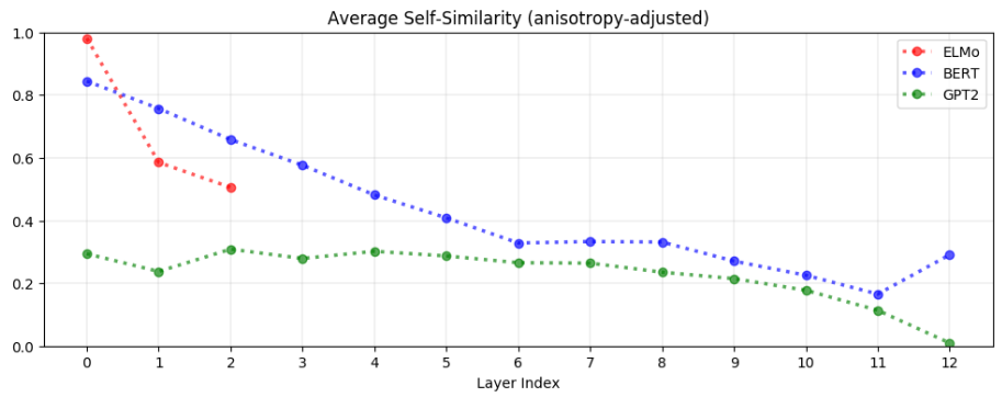
Fig. 23.1 In almost all layers of BERT and GPT-2, the word representations are anisotropic (i.e., not directionally uniform): the average cosine similarity between uniformly randomly sampled words is non-zero.

23.2.2. Context-specificity

For example, the word dog appears in A panda dog is running on the road and A dog is trying to get bacon off his back. If a model generated the same representation for dog in both these sentences, we could infer that there was no contextualization; conversely, if the two representations were different, we could infer that they were contextualized to some extent.

It is found that:

• Contextualized word embeddings are more context-specific in higher layers. Particularly, representations in GPT-2 are the most context-specific, with those in GPT-2’s last layer being almost maximally context-specific.

In image classification models, lower layers recognize more generic features such as edges while upper layers recognize more class-specific features.

Therefore, it follows that upper layers of neural language models learn more context-specific representations, so as to predict the next word for a given context more accurately.

• Stopwords (e.g., the, of, to) have among the most context-specific representations, meaning that their representation are highly dependent on its context.

23.2.3. Static vs Contextual Word embeddings

A word’s embedding changes when the word resides in different contexts. It is found that, on average, less than 5% of such variance can be explained by the first principal component, which can be viewed as a static embedding. This also indicates that contextually word embedding cannot be easily replaced by a static embedding.

However, we can still use principal components of contextualized representations in lower layers as proxy static word embeddings, which can be used in low-resource scenarios. It is found [Eth19] that such proxy static embedding can still outperform GloVe and FastText on many benchmarks.

We can create static embeddings for each word by taking the first principal component (PC) of its contextualized representations in a given layer.

Given that upper layers are much more contextspecific than lower layers, and given that GPT2’s representations are more context-specific than ELMo and BERT’s (see Figure 2), this suggests that the PCs of highly context-specific representations are less effective on traditional benchmarks.

[WHH+19]

23.3. Contrastive Learning Fundamentals

23.3.1. coSENTLoss

Following the prior study (Su, 2022), we employ the cosine objective function for end-to-end optimization of cosine similarity between representations, as follows:

\[ \mathcal{L}_{\text {cos }}=\log \left[1+\sum_{s\left(\mathbf{X}_i, \mathbf{X}_j\right)>s\left(\mathbf{X}_m, \mathbf{X}_n\right)} \exp{\left(\cos \left(\mathbf{X}_m, \mathbf{X}_n\right)-\cos \left(\mathbf{X}_i, \mathbf{x}_j\right)\right)/\tau}\right] \]

where \(\tau\) is a temperature hyperparameter, \(\cos (\cdot)\) is the cosine similarity function, and \(s(u, v)\) is the similarity between \(u\) and \(v\). By optimizing the \(\mathcal{L}_{\text {cos }}\), we expect the cosine similarity of the high similarity pair to be greater than that of the low similarity pair.

23.3.2. Embedding quality intrinsic measurement

Embedding quality, often as a result of contrastive learning, can be intrinsically measured using two properties: Alignment and uniformity [WI20]. Given a distribution of positive pairs \(p_{\text {pos }}\), alignment calculates expected distance between embeddings of the paired instances (assuming representations are already normalized):

\[ \ell_{\mathrm{align}} \triangleq \underset{\left(x, x^{+}\right) \sim p_{\mathrm{pos}}}{\mathbb{E}}\left\|f(x)-f\left(x^{+}\right)\right\|^2 \]

On the other hand, uniformity measures how well the embeddings are uniformly distributed:

\[\begin{split} \ell_{\text {uniform }} \triangleq \log \underset{\substack{\text { i.i.d. } \\ x, y \sim p_{\text {data }}}}{\mathbb{E}} \quad e^{-2\|f(x)-f(y)\|^2} \end{split}\]

where \(p_{\text {data }}\) denotes the data distribution. These two metrics are well aligned with the objective of contrastive learning: positive instances should stay close and embeddings for random instances should scatter on the hypersphere. In the following sections, we will also use the two metrics to justify the inner workings of our approaches.

23.3.3. Anisotropy problem in embeddings

[Eth19]

Recent work identifies an anisotropy problem in language representations (Ethayarajh, 2019; Li et al., 2020), i.e., the learned embeddings occupy a narrow cone in the vector space, which severely limits their expressiveness.

Wang et al. (2020) show that singular values of the word embedding matrix in a language model decay drastically: except for a few dominating singular values, all others are close to zero.

The anisotropy problem is naturally connected to uniformity (Wang and Isola, 2020), both highlighting that embeddings should be evenly distributed in the space. Intuitively, optimizing the contrastive learning objective can improve uniformity (or ease the anisotropy problem), as the objective pushes negative instances apart.

23.4. Transformer based embeddings

23.4.1. Sentence-BERT

While a pretrained BERT has provided contextulized embeddings for each token, it is found that high-quality, semantically meaning sentence embeddings can not be directly derived from token embedding.

Sentence-BERT [RG19] enables sentence embedding extraction from the BERT model after fine-tuning the BERT model via Siamese type of learningFig. 23.2. Specifically, three strategies can be used to derived sentence embedding

• the output of the CLS-token

• the mean of all output vectors (default)

• max-over-time of the output vectors

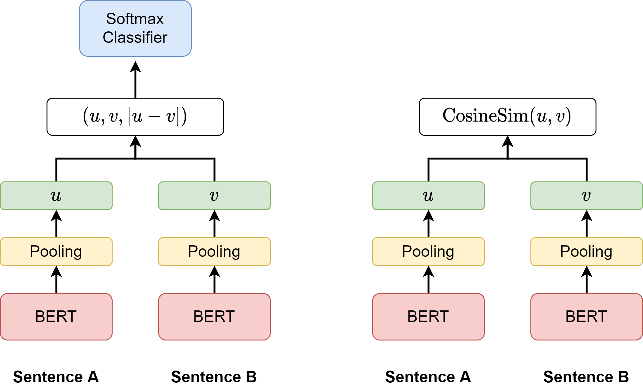
Fig. 23.2 (left) Sentence-BERT architecture with classification objective function for training. The two BERT networks are pre-trained have tied weights (Siamese network structure). (right) Sentence-BERT architecture at inference. The similarity between two input sentences can be computed as the similarity score between two sentence embeddings.

Model	Spearman
Avg. GloVe embeddings	58.02
Avg. BERT embeddings	46.35
SBERT-NLI-base	77.03
SBERT-NLI-base + STSb FT	85.35

Remark 23.2 (Training time and inference time inconsistency)

In the inference time, the pooled embeddings from the last layer are directly used in cosine similarity scoring. In the training time, the pooled embeddings plus its difference vector are passed through an MLP network first and then make prediction. The pooled embeddings are not optimized directly towards cosine similarity scoring. This issue is discussed in coSENTLoss

23.4.2. SimCSE

SimCSE [GYC21] introduces a simple Dropout strategy to identify positive examples and conduct unsupervised learning. As shown in Fig. 23.3,

• Positive example pairs can be constructed by passing one sentence passing through the encoder network with different dropout masking.

• Negative example pairs are coming from in-batch negatives.

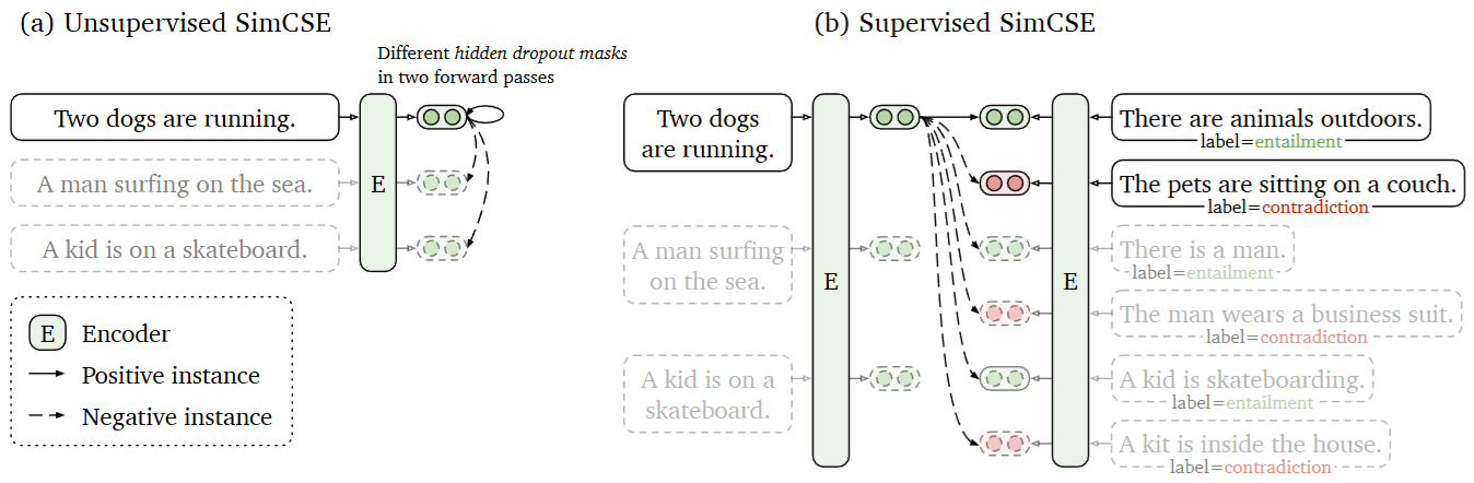
Fig. 23.3 (Left) Unsupervised SimCSE predicts the input sentence itself from in-batch negatives, with different hidden dropout masks applied. (Right) Supervised SimCSE leverages the NLI datasets and takes the entailment (premisehypothesis) pairs as positives, and contradiction pairs as well as other in-batch instances as negatives.

Contrastive learning aims to learn effective representation by pulling semantically close neighbors together and pushing apart non-neighbors (Hadsell et al., 2006). It assumes a set of paired examples \(\mathcal{D}=\left\{\left(x_{i}, x_{i}^{+}\right)\right\}_{i=1}^{m}\), where \(x_{i}\) and \(x_{i}^{+}\)are semantically related. with in-batch negatives

let \(\mathbf{h}_{i}\) and \(\mathbf{h}_{i}^{+}\)denote the representations of \(x_{i}\) and \(x_{i}^{+}\), the training objective for \(\left(x_{i}, x_{i}^{+}\right)\)with a mini-batch of \(N\) pairs is:

\[ \ell_{i}=-\log \frac{e^{\operatorname{sim}\left(\mathbf{h}_{i}, \mathbf{h}_{i}^{+}\right) / \tau}}{\sum_{j=1}^{N} e^{\operatorname{sim}\left(\mathbf{h}_{i}, \mathbf{h}_{j}^{+}\right) / \tau}} \]

where \(\tau\) is a temperature hyperparameter and \(\operatorname{sim}\left(\mathbf{h}_{1}, \mathbf{h}_{2}\right)\) is the cosine similarity \(\frac{\mathbf{h}_{1}^{\top} \mathbf{h}_{2}}{\left\|\mathbf{h}_{1}\right\| \cdot\left\|\mathbf{h}_{2}\right\|}.\)

supervised contrastive learning with hard negatives

Finally, we further take the advantage of the NLI datasets by using its contradiction pairs as hard negatives. In NLI datasets, given one premise, annotators are required to manually write one sentence that is absolutely true (entailment), one that might be true (neutral), and one that is definitely false (contradiction). Therefore, for each premise and its entailment hypothesis, there is an accompanying contradiction hypothesis.

Formally, we extend \(\left(x_{i}, x_{i}^{+}\right)\)to \(\left(x_{i}, x_{i}^{+}, x_{i}^{-}\right)\), where \(x_{i}\) is the premise, \(x_{i}^{+}\)and \(x_{i}^{-}\)are entailment and contradiction hypotheses. The training objec- tive \(\ell_{i}\) is then defined by \(N\) is mini-batch size

\[-\log \frac{e^{\operatorname{sim}\left(\mathbf{h}_{i}, \mathbf{h}_{i}^{+}\right) / \tau}}{\sum_{j=1}^{N}\left(e^{\operatorname{sim}\left(\mathbf{h}_{i}, \mathbf{h}_{j}^{+}\right) / \tau}+e^{\operatorname{sim}\left(\mathbf{h}_{i}, \mathbf{h}_{j}^{-}\right) / \tau}\right)}\]

Table 23.2 Effects of different dropout probabilities \(p\) (from 0.0 to 0.5) on the STS-B development set (Spearman’s correlation). Fixed 0.1: default 0.1 dropout rate but apply the same dropout mask on both \(x_i\) and \(x_i^{+}\).

\(p\)	0.0	0.01	0.05	0.1
STS-B	71.1	72.6	81.1	\(\mathbf{8 2 . 5}\)
\(p\)	0.15	0.2	0.5	Fixed 0.1
STS-B	81.4	80.5	71.0	43.6

23.4.2.1. CERT

\cite{fang2020cert}

CERT: Contrastive self-supervised Encoder Representations from Transformers, which pretrains language representation models using contrastive selfsupervised learning at the sentence level. CERT creates augmentations of original sentences using back-translation. Then it finetunes a pretrained language encoder (e.g., BERT) by predicting whether two augmented sentences originate from the same sentence.

CERT takes a pretrained language representation model (e.g., BERT) and finetunes it using contrastive self-supervised learning on the input data of the target task.

Fig. 23.4 The workflow of CERT. Given the large-scale input texts (without labels) from source tasks, a BERT model is first pretrained on these texts. Then we continue to train this pretrained BERT model using CSSL on the input texts (without labels) from the target task. We refer to this model as pretrained CERT model. Then we finetune the CERT model using the input texts and their associated labels in the target task and get the final model that performs the target task.

23.4.3. Sentence T5

Authors from [NAC+21] nvestigated three methods for extracting T5 sentence embeddings: two utilize only the T5 encoder and one uses the full T5 encoder-decoder model.

• Encoder-only first (ST5-Enc first): The encoder output of the first token is taken as the sentence embedding.

• Encoder-only mean (ST5-Enc mean): The sentence embedding is defined as the average of the encoder outputs across all input tokens.

• Encoder-Decoder first (ST5-EncDec first): The first decoder output is taken as the sentence embedding. To obtain the decoder output, the input text is fed into the encoder, and the standard “start” symbol is fed as the first decoder input.

Key findings are:

• Under zero-shot transfer, ST5 performs better than BERT, probabily due to the fact that T5 is pretrained on a much larger and diverse dataset.

• Using T5 encoder with mean pooling can yield generally better embeddings than the other two options.

• Further fine-tuning in labeled data can further improve the performance.

Model	Avg
BERT (CLS-vector)	84.66
BERT (mean)	84.94
ST5-Enc first	83.38
ST5-Enc mean	\(\mathbf{8 8 . 9 6}\)
ST5-EncDec first	81.69

| Model | Finetune Data | Avg | | :—: | -:–: | —: | |SBERT-NLI | NLI + MNLI | 87.41 | | ST5-Enc mean | NLI | 88.66 |

Additionally scaling up the model size can bring additional performance boost Fig. 23.5; in terms of measuring embedding quality via uniformity and alignement, when models scale up, both the encoder and encoder-decoder models decrease the uniformity loss with only a slight increase in alignment loss, as shown in {numref}``

Fig. 23.5 Scaling up ST5 model size improves performance on SentEval (left) and STS (right). Image from [NAC+21].

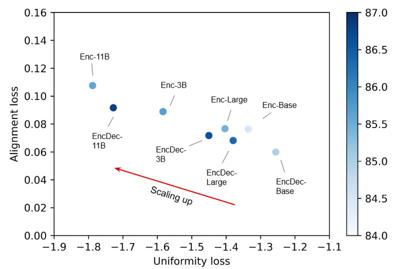
Fig. 23.6 Scaling up ST5 model size improves uniformality and alignment. Image from [NAC+21].

23.4.4. Benchmark dataset

23.4.4.1. MultiNLI data

[WNB17]

The Multi-Genre Natural Language Inference (MultiNLI) corpus ^{[^3]} is a dataset designed for use in the development and evaluation of machine learning models for sentence understanding. It has over 433,000 examples and is one of the largest datasets available for natural language inference (a.k.a recognizing textual entailment). The dataset is also designed so that existing machine learning models trained on the Stanford NLI corpus can also be evaluated using MultiNLI.

23.4.4.2. Standard semantic textual similarity tasks

[ABC+15, ABC+14, ABC+16, ACDGA12, ACD+13, CDA+17]

23.5. Knowledge Transfer and Distillation

23.5.1. From mono language to multi lingual

[RG20]

23.6. Matryoshka Representation Learning

new state-of-the-art (text) embedding models started producing embeddings with increasingly higher output dimensions, i.e., every input text is represented using more values. Although this improves performance, it comes at the cost of efficiency of downstream tasks such as search or classification.

[KBR+22]

These Matryoshka embedding models are trained such that these small truncated embeddings would still be useful. In short, Matryoshka embedding models can produce useful embeddings of various dimensions.

Matryoshka embedding models aim to store more important information in earlier dimensions, and less important information in later dimensions. This characteristic of Matryoshka embedding models allows us to truncate the original (large) embedding produced by the model, while still retaining enough of the information to perform well on downstream tasks.

For Matryoshka Embedding models, the training aims to optimize the quality of your embeddings at various different dimensionalities. For example, output dimensionalities are 768, 512, 256, 128, and 64. The loss values for each dimensionality are added together, resulting in a final loss value. The optimizer will then try and adjust the model weights to lower this loss value.

In practice, this incentivizes the model to frontload the most important information at the start of an embedding, such that it will be retained if the embedding is truncated.

23.6.1. Loss Function

For MRL, we choose \(\mathcal{M}=\{8,16, \ldots, 1024,2048\}\) as the nesting dimensions. Suppose we are given a labelled dataset \(\mathcal{D}=\left\{\left(x_1, y_1\right), \ldots,\left(x_N, y_N\right)\right\}\) where \(x_i \in \mathcal{X}\) is an input point and \(y_i \in[L]\) is the label of \(x_i\) for all \(i \in[N]\). MRL optimizes the multi-class classification loss for each of the nested dimension \(m \in \mathcal{M}\) using standard empirical risk minimization using a separate linear classifier, parameterized by \(\mathbf{W}^{(m)} \in \mathbb{R}^{L \times m}\). All the losses are aggregated after scaling with their relative importance \(\left(c_m \geq 0\right)_{m \in \mathcal{M}}\) respectively. That is, we solve

\[ \min_{\left\{\mathbf{W}^{(m)}\right\}_{m \in \mathcal{M}}} \frac{1}{N} \sum_{i \in[N]} \sum_{m \in \mathcal{M}} c_m \cdot \mathcal{L}\left(\mathbf{W}^{(m)} \cdot h_i^{1: m} ; y_i\right) \]

where \(\mathcal{L}: \mathbb{R}^L \times[L] \rightarrow \mathbb{R}_{+}\)is the multi-class softmax cross-entropy loss function. This is a standard optimization problem that can be solved using sub-gradient descent methods. We set all the importance scales, \(c_m=1\) for all \(m \in \mathcal{M}\); see Section 5 for ablations. Lastly, despite only optimizing for \(O(\log (d))\) nested dimensions, MRL results in accurate representations, that interpolate, for dimensions that fall between the chosen granularity of the representations (Section 4.2).

23.7. General-Purpose Text Embedding

23.7.1. Overview

General-purpose text embedding aims to be a strong performing single-vector representation that can be applied in a broad range of tasks in both zero-shot or fine-tuned settings.

The quality and diversity of the training data is crucial for training general-purpose text embeddings.

Model training usually consists of multiple stages, including

• A large scale unsupervised or weakly supervised contrastive learning

• A small scale supervised constrastive learning.

23.7.2. E5 and mE5

A crucial step for E5 contrastive pre-training is data collection and quality control.

The authors created a text pair dataset called CCPairs (Colossal Clean text Pairs) by harvesting heterogeneous semi-structured data sources. Let \((q, p)\) denote a text pair consisting of a query \(q\) and a passage \(p\). Here we use “passage” to denote word sequences of arbitrary length, which can be a short sentence, a paragraph, or a long document. The dataset includes

Data Source	Text Pair
Reddit	(post, comment)
Stackexchange	(question, upvoted answer)
English Wikipedia	(entity name + section title, passage)
Scientific papers	(title, abstract) and citation
Common Crawl	(title, passage)
News sources	(title, passage)

Additional rule-based filtering steps are applied to Reddit and Common Crawl. For example, we remove Reddit comments that are either too long ( \(>4096\) characters) or receive score less than 1 , and remove passages from web pages with high perplexity. This yielded about 1.3B text pairs.

Then, consistency-based filter is further used for quality improvement: a model is first trained on the 1.3 B noisy text pairs, and then used to rank each pair against a pool of 1 million random passages. A text pair is kept only if it falls in the top- \(k\) (k=2) ranked lists. This step led to \(\sim 270 \mathrm{M}\) text pairs for contrastive pre-training.

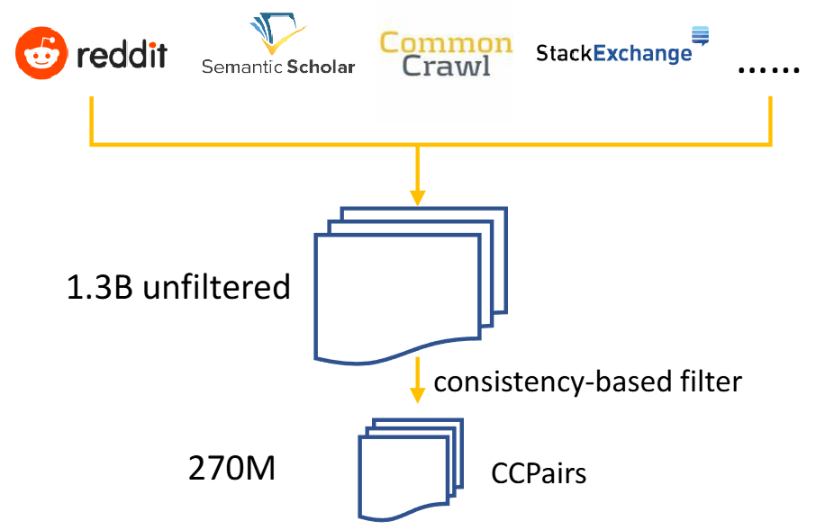
Fig. 23.7 Contrastive pretraining data curation process for E5. Image from [WYH+22].

Supervised finetuning

While contrastive pre-training on the CCPairs provides a solid foundation for general-purpose embeddings, further training on labeled data can inject human knowledge into the model to boost the performance.

Data Source	Target Domain
NLI	Semantic textual similarity
NQ	Text retrieval
MS MARCO	Text retrieval

| English Wikipedia | (entity name + section title, passage) | | Scientific papers| (title, abstract) and citation| | Common Crawl | (title, passage) | | News sources | (title, passage) |

Although these datasets are small, existing works [43, 44] have shown that supervised fine-tuning leads to consistent performance gains. In this paper, we choose to further train with a combination of 3 datasets: NLI \({ }^6\) (Natural Language Inference), MS-MARCO passage ranking dataset [8], and NQ (Natural Questions) dataset [30, 32]. Empirically, tasks like STS (Semantic Textual Similarity) and linear probing benefit from NLI data, while MS-MARCO and NQ datasets transfer well to retrieval tasks. Building on the practices of training state-of-the-art dense retrievers [50,58], we use mined hard negatives and knowledge distillation from a cross-encoder (CE) teacher model for the MS-MARCO and NQ datasets. For the NLI dataset, contradiction sentences are regarded as hard negatives. The loss function is a linear interpolation between contrastive loss \(L_{\text {cont }}\) for hard labels and KL divergence \(D_{\mathrm{KL}}\) for distilling soft labels from the teacher model.

\[ \min D_{\mathrm{KL}}\left(p_{\mathrm{ce}}, p_{\mathrm{stu}}\right)+\alpha L_{\mathrm{cont}} \]

Where \(p_{\text {ce }}\) and \(p_{\text {stu }}\) are the probabilities from the cross-encoder teacher model and our student model. \(\alpha\) is a hyperparameter to balance the two loss functions. \(L_{\text {cont }}\) is the same as in Equation 1.

	BM25 \(^2\)	SimCSE	Contriever	E5-PT \(_{\text {small }}\)	E5-PT \(_{\text {base }}\)	E5-PT \(_{\text {largc }}\)
MS MARCO	22.8	9.4	20.6	25.4	26.0	26.2
BEIR (Avg)	41.7	20.3	36.0	40.8	42.9	44.2

[WYH+24]

| | ANCE | GTR \(_{\text {base }}\) | ColBERT | Contriever | GTR \(_{\text {large }}\) | E5 \(_{\text {small }}\) | E5 \(_{\text {base }}\) | E5 \(_{\text {large }}\) | | :—: | :—: | :—: | :—: | :—: | :—: | :—: | :—: | :—: | :—: | | MS MARCO | 38.8 | 42.0 | 40.1 | 40.7 | 43.0 | 42.3 | 43.1 | 44.1 | | Average | 40.5 | 44.0 | 44.4 | 46.6 | 47.0 | 46.0 | 48.7 | 50.0 |

23.7.3. GTE

23.8. Software

haystack

23.9. Bibliography

[ABC+15]

Eneko Agirre, Carmen Banea, Claire Cardie, Daniel Cer, Mona Diab, Aitor Gonzalez-Agirre, Weiwei Guo, Inigo Lopez-Gazpio, Montse Maritxalar, Rada Mihalcea, and others. Semeval-2015 task 2: semantic textual similarity, english, spanish and pilot on interpretability. In Proceedings of the 9th international workshop on semantic evaluation (SemEval 2015), 252–263. 2015.

[ABC+14]

Eneko Agirre, Carmen Banea, Claire Cardie, Daniel M Cer, Mona T Diab, Aitor Gonzalez-Agirre, Weiwei Guo, Rada Mihalcea, German Rigau, and Janyce Wiebe. Semeval-2014 task 10: multilingual semantic textual similarity. In SemEval@ COLING, 81–91. 2014.

[ABC+16]

Eneko Agirre, Carmen Banea, Daniel Cer, Mona Diab, Aitor Gonzalez Agirre, Rada Mihalcea, German Rigau Claramunt, and Janyce Wiebe. Semeval-2016 task 1: semantic textual similarity, monolingual and cross-lingual evaluation. In SemEval-2016. 10th International Workshop on Semantic Evaluation; 2016 Jun 16-17; San Diego, CA. Stroudsburg (PA): ACL; 2016. p. 497-511. ACL (Association for Computational Linguistics), 2016.

[ACDGA12]

Eneko Agirre, Daniel Cer, Mona Diab, and Aitor Gonzalez-Agirre. Semeval-2012 task 6: a pilot on semantic textual similarity. In * SEM 2012: The First Joint Conference on Lexical and Computational Semantics–Volume 1: Proceedings of the main conference and the shared task, and Volume 2: Proceedings of the Sixth International Workshop on Semantic Evaluation (SemEval 2012), 385–393. 2012.

[ACD+13]

Eneko Agirre, Daniel Cer, Mona Diab, Aitor Gonzalez-Agirre, and Weiwei Guo. * sem 2013 shared task: semantic textual similarity. In Second joint conference on lexical and computational semantics (* SEM), volume 1: proceedings of the Main conference and the shared task: semantic textual similarity, 32–43. 2013.

[BAPM15]

Samuel R Bowman, Gabor Angeli, Christopher Potts, and Christopher D Manning. A large annotated corpus for learning natural language inference. arXiv preprint arXiv:1508.05326, 2015.

[CDA+17] (1,2)

Daniel Cer, Mona Diab, Eneko Agirre, Inigo Lopez-Gazpio, and Lucia Specia. Semeval-2017 task 1: semantic textual similarity-multilingual and cross-lingual focused evaluation. arXiv preprint arXiv:1708.00055, 2017.

[DB05]

William B Dolan and Chris Brockett. Automatically constructing a corpus of sentential paraphrases. In Proceedings of the Third International Workshop on Paraphrasing (IWP2005). 2005.

[Eth19] (1,2,3)

Kawin Ethayarajh. How contextual are contextualized word representations? comparing the geometry of bert, elmo, and gpt-2 embeddings. arXiv preprint arXiv:1909.00512, 2019.

[GHT+19]

Jun Gao, Di He, Xu Tan, Tao Qin, Liwei Wang, and Tie-Yan Liu. Representation degeneration problem in training natural language generation models. arXiv preprint arXiv:1907.12009, 2019.

[GYC21]

Tianyu Gao, Xingcheng Yao, and Danqi Chen. Simcse: simple contrastive learning of sentence embeddings. arXiv preprint arXiv:2104.08821, 2021.

[KBR+22]

Aditya Kusupati, Gantavya Bhatt, Aniket Rege, Matthew Wallingford, Aditya Sinha, Vivek Ramanujan, William Howard-Snyder, Kaifeng Chen, Sham Kakade, Prateek Jain, and others. Matryoshka representation learning. Advances in Neural Information Processing Systems, 35:30233–30249, 2022.

[NAC+21] (1,2,3)

Jianmo Ni, Gustavo Hernandez Abrego, Noah Constant, Ji Ma, Keith B Hall, Daniel Cer, and Yinfei Yang. Sentence-t5: scalable sentence encoders from pre-trained text-to-text models. arXiv preprint arXiv:2108.08877, 2021.

[RG19]

Nils Reimers and Iryna Gurevych. Sentence-bert: sentence embeddings using siamese bert-networks. arXiv preprint arXiv:1908.10084, 2019.

[RG20]

Nils Reimers and Iryna Gurevych. Making monolingual sentence embeddings multilingual using knowledge distillation. arXiv preprint arXiv:2004.09813, 2020.

[WYH+22]

Liang Wang, Nan Yang, Xiaolong Huang, Binxing Jiao, Linjun Yang, Daxin Jiang, Rangan Majumder, and Furu Wei. Text embeddings by weakly-supervised contrastive pre-training. arXiv preprint arXiv:2212.03533, 2022.

[WYH+24]

Liang Wang, Nan Yang, Xiaolong Huang, Linjun Yang, Rangan Majumder, and Furu Wei. Multilingual e5 text embeddings: a technical report. arXiv preprint arXiv:2402.05672, 2024.

[WHH+19]

Lingxiao Wang, Jing Huang, Kevin Huang, Ziniu Hu, Guangtao Wang, and Quanquan Gu. Improving neural language generation with spectrum control. In International Conference on Learning Representations. 2019.

[WI20]

Tongzhou Wang and Phillip Isola. Understanding contrastive representation learning through alignment and uniformity on the hypersphere. In International Conference on Machine Learning, 9929–9939. PMLR, 2020.

[WNB17]

Adina Williams, Nikita Nangia, and Samuel R Bowman. A broad-coverage challenge corpus for sentence understanding through inference. arXiv preprint arXiv:1704.05426, 2017.