24. Information Retrieval and Dense Models#
24.1. Semantic Dense Models#
24.1.1. Motivation#
For ad-hoc search, traditional exact-term matching models (e.g., BM25) are playing critical roles in both traditional IR systems [Fig. 23.5] and modern multi-stage pipelines [Fig. 23.6]. Unfortunately, exact-term matching inherently suffers from the vocabulary mismatch problem due to the fact that a concept is often expressed using different vocabularies and language styles in documents and queries.
Early latent semantic models such as latent semantic analysis (LSA) illustrated the idea of identifying semantically relevant documents for a query when lexical matching is insufficient. However, their effectiveness in addressing the language discrepancy between documents and search queries are limited by their weak modeling capacity (i.e., simple, linear models). Also, these model parameters are typically learned via the unsupervised learning, i.e., by grouping different terms that occur in a similar context into the same semantic cluster.
The introduction of deep neural networks for semantic modeling and retrieval was pioneered in [HHG+13]. Recent deep learning model utilize the neural networks with large learning capacity and user-interaction data for supervised learning, which has led to significance performance gain over LSA. Similarly in the field of OpenQA [KOuguzM+20], whose first stage is to retrieve relevant passages that might contain the answer, semantic-based retrieval has also demonstrated performance gains over traditional retrieval methods.
24.1.2. Two Architecture Paradigms#
The current neural architecture paradigms for IR can be categorized into two classes: representation-based and interaction-based [Fig. 24.1].
In the representation-based architecture, a query and a document are encoded independently into two embedding vectors, then their relevance is estimated based on a single similarity score between the two embedding vectors.
Here we would like to make a critical distinction on symmetric vs. asymmetric encoding:
For symmetric encoding, the query and the entries in the corpus are typically of the similar length and have the same amount of content and they are encoded using the same network. Symmetric encoding is used for symmetric semantic search. An example would be searching for similar questions. For instance, the query could be How to learn Python online? and the entry that satisfies the search is like How to learn Python on the web?.
For asymmetric encoding, we usually have a short query (like a question or some keywords) and we would like to find a longer paragraph answering the query; they are encoded using two different networks. An example would be information retrieval. The entry is typically a paragraph or a web-page.
In the interaction-based architecture, instead of directly encoding \(q\) and \(d\) into individual embeddings, term-level interaction features across the query and the document are first constructed. Then a deep neural network is used to extract high-level matching features from the interactions and produce a final relevance score.
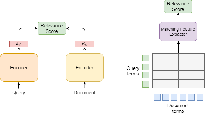
Fig. 24.1 Two common architectural paradigms in semantic retrieval learning: representation-based learning (left) and interaction-based learning (right).#
These two architectures have different strengths in modeling relevance and final model serving. For example, a representation-based model architecture makes it possible to pre-compute and cache document representations offline, greatly reducing the online computational load per query. However, the pre-computation of query-independent document representations often miss term-level matching features that are critical to construct high-quality retrieval results. On the other hand, interaction-based architectures are often good at capturing the fine-grained matching feature between the query and the document.
Since interaction-based models can model interactions between word pairs in queries and document, they are effective for re-ranking, but are cost-prohibitive for first-stage retrieval as the expensive document-query interactions must be computed online for all ranked documents.
Representation-based models enable low-latency, full-collection retrieval with a dense index. By representing queries and documents with dense vectors, retrieval is reduced to nearest neighbor search, or a maximum inner product search (MIPS) [] problem if similarity is represented by an inner product.
In recent years, there has been increasing effort on accelerating maximum inner product and nearest neighbor search, which led to high-quality implementations of libraries for nearest neighbor search such as hnsw [MY18], FAISS [JDJegou19], and SCaNN [GSL+20].
24.1.3. Classic Representation-based Learning#
24.1.3.1. DSSM#
Deep structured semantic model (DSSM) [HHG+13] improves the previous latent semantic models in two aspects:
DSSM is supervised learning based on labeled data, while latent semantic models are unsupervised learning;
DSSM utilize deep neural networks to capture more semantic meanings.
The high-level architecture of DSSM is illustrated in Fig. 24.2. First, we represent a query and a document (only its title) by a sparse vector, respectively. Second, we apply a non-linear projection to map the query and the document sparse vectors to two low-dimensional embedding vectors in a common semantic space. Finally, the relevance of each document given the query is calculated as the cosine similarity between their embedding vectors in that semantic space.
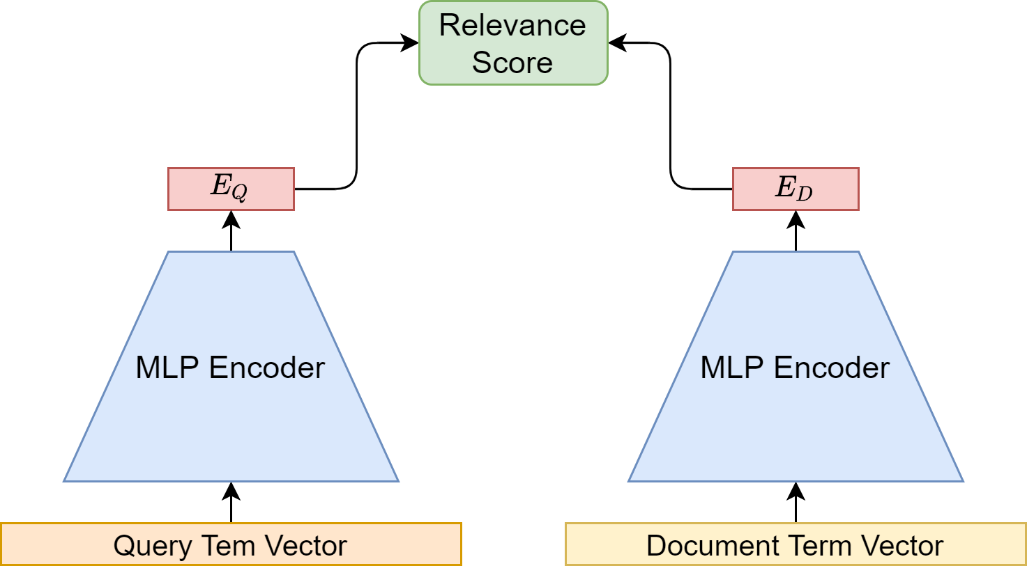
Fig. 24.2 The architecture of DSSM. Two MLP encoders with shared parameters are used to encode a query and a document into dense vectors. Query and document are both represented by term vectors. The final relevance score is computed via dot product between the query vector and the document vector.#
To represent word features in the query and the documents, DSSM adopt a word level sparse term vector representation with letter 3-gram vocabulary, whose size is approximately \(30k \approx 30^3\). Here 30 is the approximate number of alphabet letters. This is also known as a letter trigram word hashing technique. In other words, both query and the documents will be represented by sparse vectors with dimensionality of \(30k\).
The usage of letter 3-gram vocabulary has multiple benefits compared to the full vocabulary:
Avoid OOV problem with finite-size vocabulary or term vector dimensionality.
The use of letter n-gram can capture morphological meanings of words.
One problem of this method is collision, i.e., two different words could have the same letter n-gram vector representation because this is a bag-of-words representation that does not take into account orders. But the collision probability is rather low.
Word Size |
Letter-Bigram |
Letter-Trigram |
||
|---|---|---|---|---|
Token Size |
Collision |
Token Size |
Collision |
|
40k |
1107 |
18 |
10306 |
2 |
500k |
1607 |
1192 |
30621 |
22 |
Training. The neural network model is trained on the clickthrough data to map a query and its relevant document to vectors that are similar to each other and vice versa. The click-through logs consist of a list of queries and their clicked documents. It is assumed that a query is relevant, at least partially, to the documents that are clicked on for that query.
The semantic relevance score between a query \(q\) and a document \(d\) is given by:
where \(E_{q}\) and \(E_{q}\) are the embedding vectors of the query and the document, respectively. The conditional probability of a document being relevant to a given query is now defined through a Softmax function
where \(\gamma\) is a smoothing factor as a hyperparameter. \(D\) denotes the set of candidate documents to be ranked. While \(D\) should ideally contain all possible documents in the corpus, in practice, for each query \(q\), \(D\) is approximated by including the clicked document \(d^{+}\) and four randomly selected un-clicked documents.
In training, the model parameters are estimated to maximize the likelihood of the clicked documents given the queries across the training set. Equivalently, we need to minimize the following loss function
Evaluation DSSM is compared with baselines of traditional IR models like TF-IDF, BM25, and LSA. Specifically, the best performing DNN-based semantic model, L-WH DNN, uses three hidden layers, including the layer with the Letter-trigram-based Word Hashing, and an output layer, and is discriminatively trained on query-title pairs.
Models |
NDCG@1 |
NDCG@3 |
NDCG@10 |
|---|---|---|---|
TF-IDF |
0.319 |
0.382 |
0.462 |
BM25 |
0.308 |
0.373 |
0.455 |
LSA |
0.298 |
0.372 |
0.455 |
L-WH DNN |
0.362 |
0.425 |
0.498 |
24.1.3.2. CNN-DSSM#
DSSM treats a query or a document as a bag of words, the fine-grained contextual structures embedding in the word order are lost. The DSSM-CNN[SHG+14] [Fig. 24.3] directly represents local contextual features at the word n-gram level; i.e., it projects each raw word n-gram to a low dimensional feature vector where semantically similar word \(\mathrm{n}\) grams are projected to vectors that are close to each other in this feature space.
Moreover, instead of simply summing all local word-n-gram features evenly, the DSSM-CNN performs a max pooling operation to select the highest neuron activation value across all word n-gram features at each dimension. This amounts to extract the sentence-level salient semantic concepts.
Meanwhile, for any sequence of words, this operation forms a fixed-length sentence level feature vector, with the same dimensionality as that of the local word n-gram features.
Given the letter-trigram based word representation, we represent a word-n-gram by concatenating the letter-trigram vectors of each word, e.g., for the \(t\)-th word-n-gram at the word-ngram layer, we have:
where \(f_{t}\) is the letter-trigram representation of the \(t\)-th word, and \(n=2 d+1\) is the size of the contextual window. In our experiment, there are about \(30K\) unique letter-trigrams observed in the training set after the data are lower-cased and punctuation removed. Therefore, the letter-trigram layer has a dimensionality of \(n \times 30 K\).
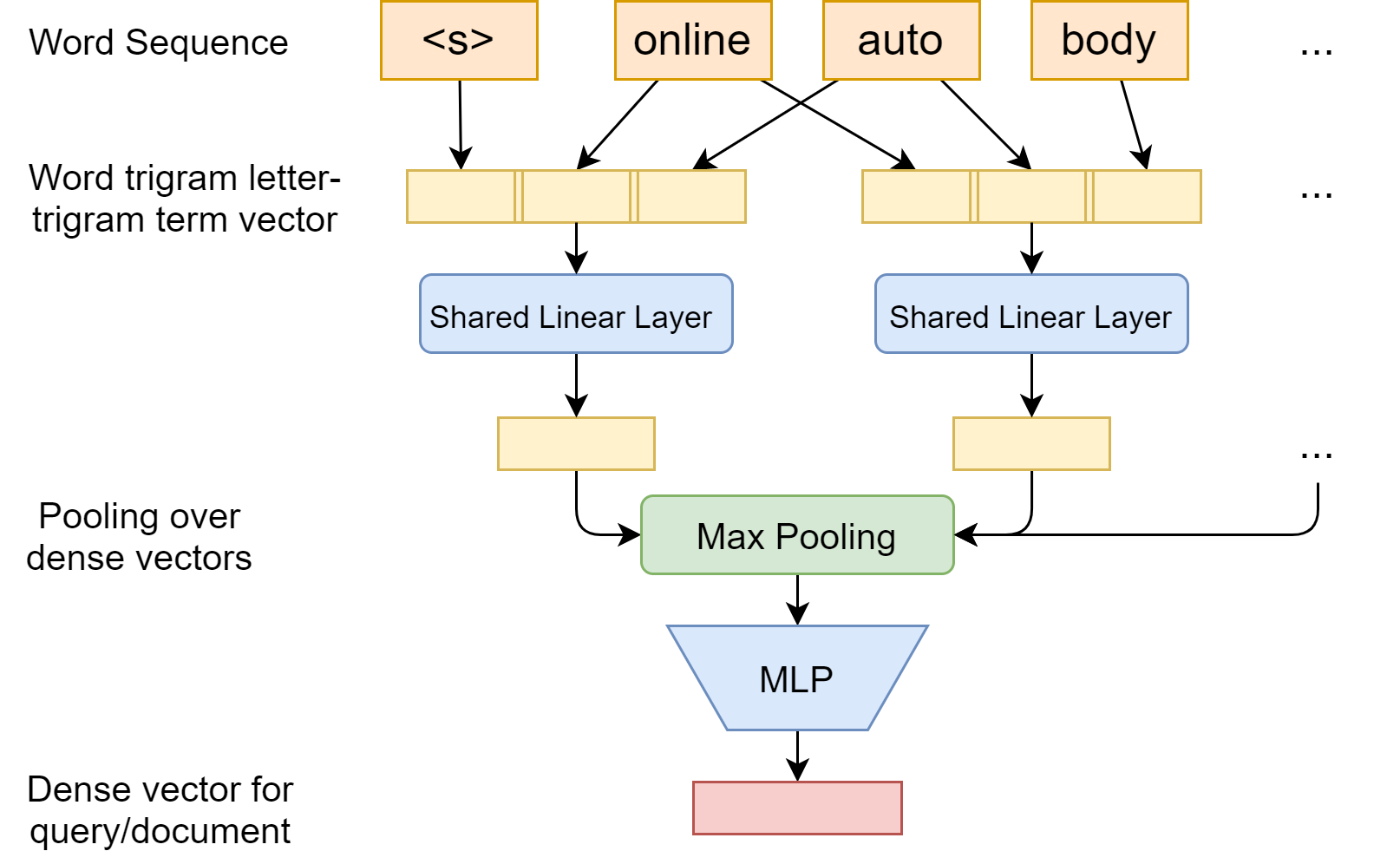
Fig. 24.3 The architecture of CNN-DSSM. Each term together with its left and right contextual words are encoded together into term vectors.#
24.2. Transfomer Retrievers and Rerankers#
24.2.1. Overview#
BERT (Bidirectional Encoder Representations from Transformers) [DCLT18] and its transformer variants [LWLQ21] represent the state-of-the-art modeling strategies in a broad range of natural language processing tasks. The application of BERT in information retrieval and ranking was pioneered by [NC19, NYCL19]. The fundamental characteristics of BERT architecture is self-attention. By pretraining BERT on large scale text data, BERT encoder can produce contextualized embeddings can better capture semantics of different linguistic units. By adding additional prediction head to the BERT backbone, such BERT encoders can be fine-tuned to retrieval related tasks.
In general, there are two mainstream architectures in using BERT for information retrieval and ranking tasks [[]].
Bi-encoder, also known as dual-encoder or twin-tower models, employ two separate encoders to generate independent embeddings for each input text segment. The relevance label is predicted using similarity scores between the query embedding and the doc embedding.
Cross-encoder, process both input text segments together within a single encoder. This joint encoding allows the model to capture richer relationships and dependencies between the text segments, leading to higher accuracy in tasks that require a deeper understanding of the semantic similarity or relatedness between the inputs.
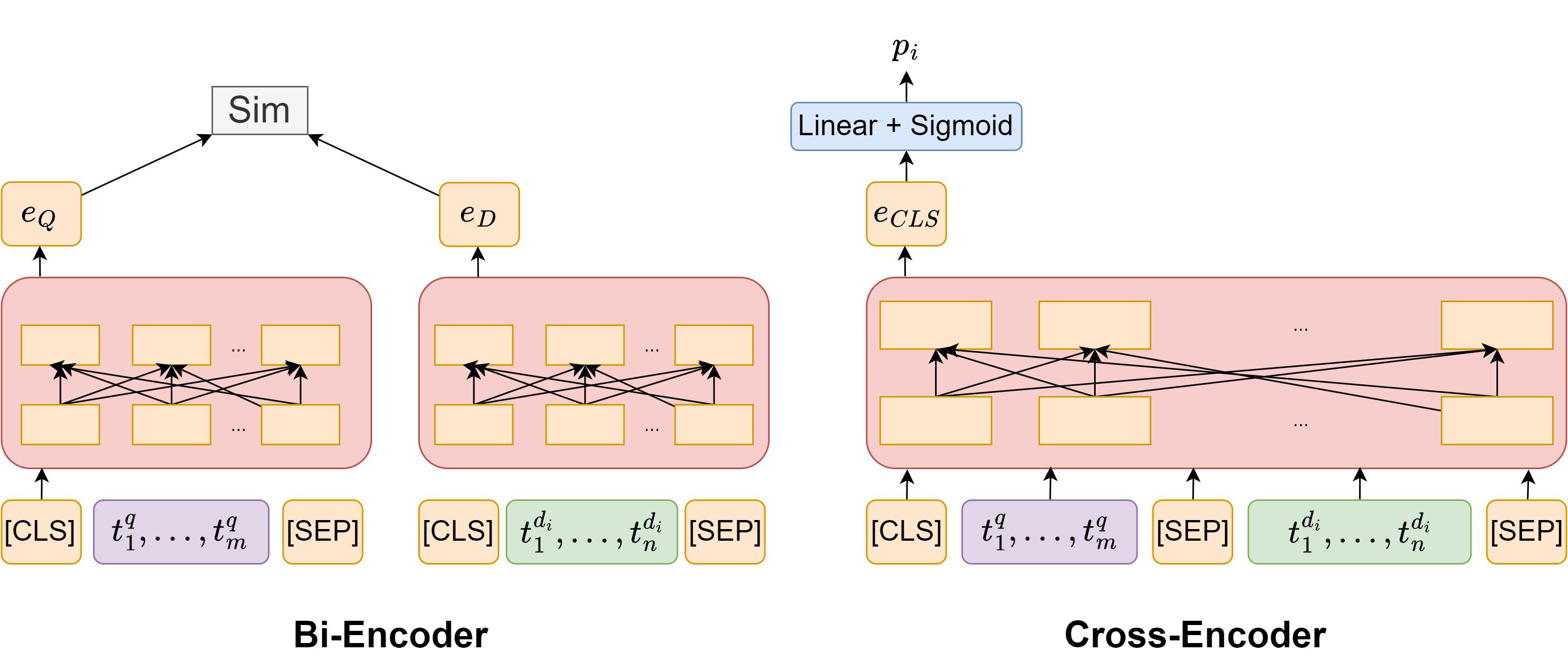
Fig. 24.4 (Left) The Bi-Encoder architecture for document relevance ranking. The query and document inputs are passed to query encoder and document encoder separately. The [CLS] embedding for query encoder and the doc encoder are used to compute similiarity score, as the proxy of relevance score. (Right) The Cross-Encoder architecture for document relevance ranking. The input is the concatenation of the query token sequence and the candidate document token sequence. Once the input sequence is passed through the model, we use the [CLS] embedding as input to a single layer neural network to obtain a posterior probability \(p_{i}\) of the candidate \(d_{i}\) being relevant to query \(q\).#
24.2.2. Bi-Encoder Retriever#
Using Bi-Encoder as retriever was first explored in passage retrieval RepBERT [ZML+20] and OpenDomain QA DPR [KOuguzM+20].
In RepBERT, the query encoder and document encoder shares the same weight. The encoding is the mean of the last hidden states of input tokens. In DPR, the query encoder and document encoder are separate encoder, and the text encoding is taking the representation at the [CLS].
The relevance score between a query and a passage is expressed as the similarity between the query and the passage embeddings, given by
Loss Function The goal of training is to make the embedding inner products of relevant pairs of queries and documents larger than those of irrelevant pairs. Let \(\left(q, d_1^{+}, \ldots, d_m^{+}, d_{m+1}^{-}, \ldots, d_n^{-}\right)\)be one instance of the input training batch. The instance contains one query \(q, m\) relevant (positive) documents and \(n-m\) irrelevant (negative) documents. We adopt MultiLabelMarginLoss [16] as the loss function:
Let \(\mathcal{D}=\left\{\left\langle q_i, p_i^{+}, p_{i, 1}^{-}, \cdots, p_{i, n}^{-}\right\rangle\right\}_{i=1}^m\) be the training data that consists of \(m\) instances. Each instance contains one question \(q_i\) and one relevant (positive) passage \(p_i^{+}\), along with \(n\) irrelevant (negative) passages \(p_{i, j}^{-}\). We optimize the loss function as the negative \(\log\) likelihood of the positive passage:
24.2.3. Cross-Encoder For Point-wise Ranking#
The first application of BERT in document retrieval is using BERT as a cross encoder, where the query token sequence and the document token sequence are concatenated via [SEP] token and encoded together. This architecture [Fig. 24.4], called mono-BERT, was first proposed by [NC19, NYCL19].
To meet the token sequence length constraint of a BERT encoder (e.g., 512), we might need to truncate the query (e.g, not greater than 64 tokens) and the candidate document token sequence such that the total concatenated token sequence have a maximum length of 512 tokens.
Once the input sequence is passed through the model, we use the [CLS] embedding as input to a single layer neural network to obtain a posterior binary classification probability \(p_{i}\) of the candidate \(d_{i}\) being relevant to query \(q\). The posterior probability can be used to rank documents.
The training data can be represented by a collections of triplets \((q, J_P^q, J_N^q), q\in Q\), where \(Q\) is the set of queries, \(J_{P}^q\) is the set of indexes of the relevant candidates associated with query \(q\) and \(J_{N}^q\) is the set of indexes of the nonrelevant candidates.
The encoder can be fine-tuned using cross-entropy loss:
where \(p_j\) is the probability that \(q\) is relevant to passage \(P\).
During training, each batch can consist of a query and its candidate documents (include both positive and negative) produced by previous retrieval layers.
24.2.4. Duo-BERT For Pairwise Ranking#
Mono-BERT can be characterized as a pointwise approach for ranking. Within the framework of learning to rank, [NC19, NYCL19] also proposed duo-BERT, which is a pairwise ranking approach. In this pairwise approach, the duo-BERT ranker model estimates the probability \(p_{i, j}\) of the candidate \(d_{i}\) being more relevant than \(d_{j}\) with respect to query \(q\).
The duo-BERT architecture [Fig. 24.5] takes the concatenation of the query \(q\), the candidate document \(d_{i}\), and the candidate document \(d_{j}\) as the input. We also need to truncate the query, candidates \(d_{i}\) and \(d_{j}\) to proper lengths (e.g., 62 , 223 , and 223 tokens, respectively), so the entire sequence will have at most 512 tokens.
Once the input sequence is passed through the model, we use the [CLS] embedding as input to a single layer neural network to obtain a posterior probability \(p_{i,j}\). This posterior probability can be used to rank documents \(i\) and \(j\) with respect to each other. If there are \(k\) candidates for query \(q\), there will be \(k(k-1)\) passes to compute all the pairwise probabilities.
The model can be fine-tune using with the following loss per query.
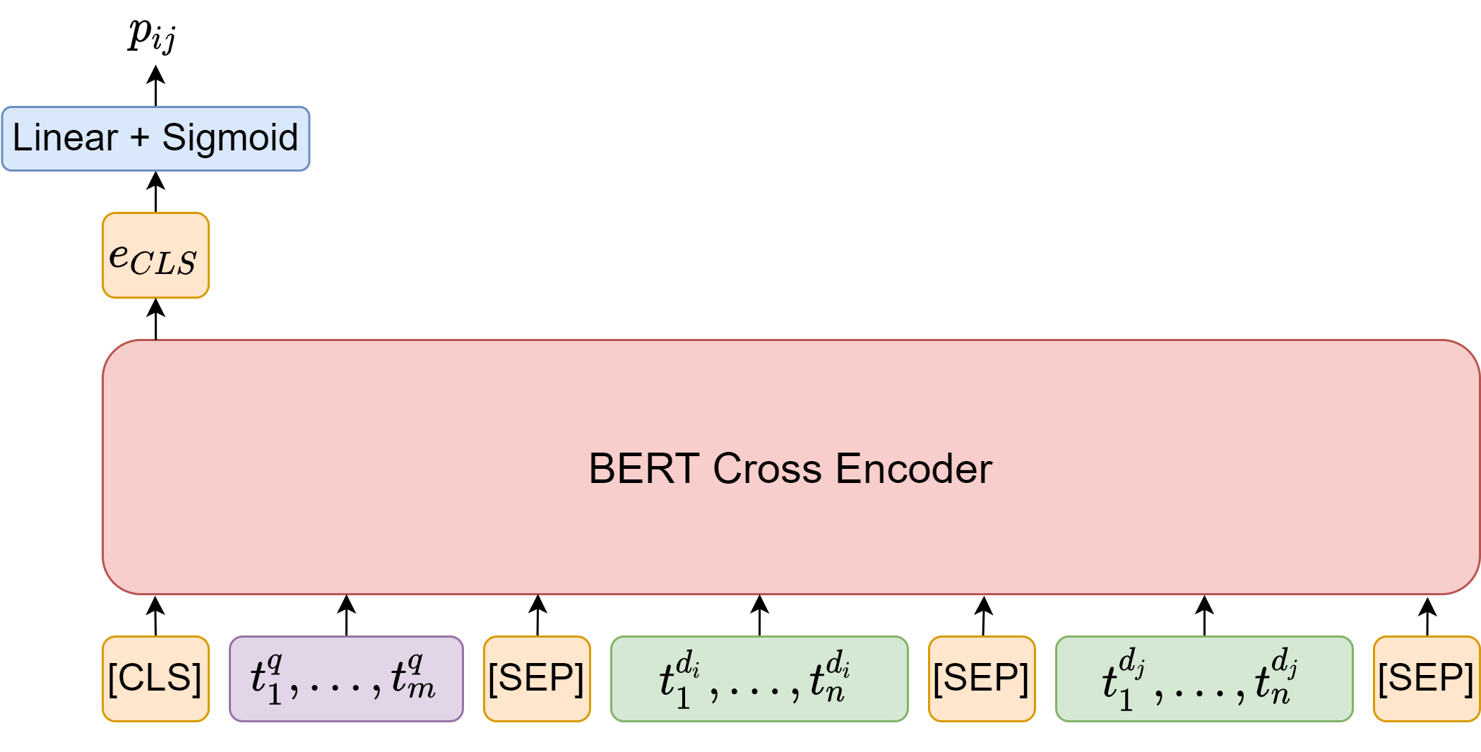
Fig. 24.5 The duo-BERT architecture takes the concatenation of the query and two candidate documents as the input. Once the input sequence is passed through the model, we use the [CLS] embedding as input to a single layer neural network to obtain a posterior probability that the first document is more relevant than the second document.#
At inference time, the obtained \(k(k -1)\) pairwise probabilities are used to produce the final document relevance ranking given the query. Authors in [NYCL19] investigate five different aggregation methods (SUM, BINARY, MIN, MAX, and SAMPLE) to produce the final ranking score.
where \(J_i = \{1 <= j <= k, j\neq i\}\) and \(J_i(m)\) is \(m\) randomly sampled elements from \(J_i\).
The SUM method measures the pairwise agreement that candidate \(d_{i}\) is more relevant than the rest of the candidates \(\left\{d_{j}\right\}_{j \neq i^{*}}\). The BINARY method resembles majority vote. The Min (MAX) method measures the relevance of \(d_{i}\) only against its strongest (weakest) competitor. The SAMPLE method aims to decrease the high inference costs of pairwise computations via sampling. Comparison studies using MS MARCO dataset suggest that SUM and BINARY give the best results.
24.2.5. Multistage Retrieval and Ranking Pipeline#
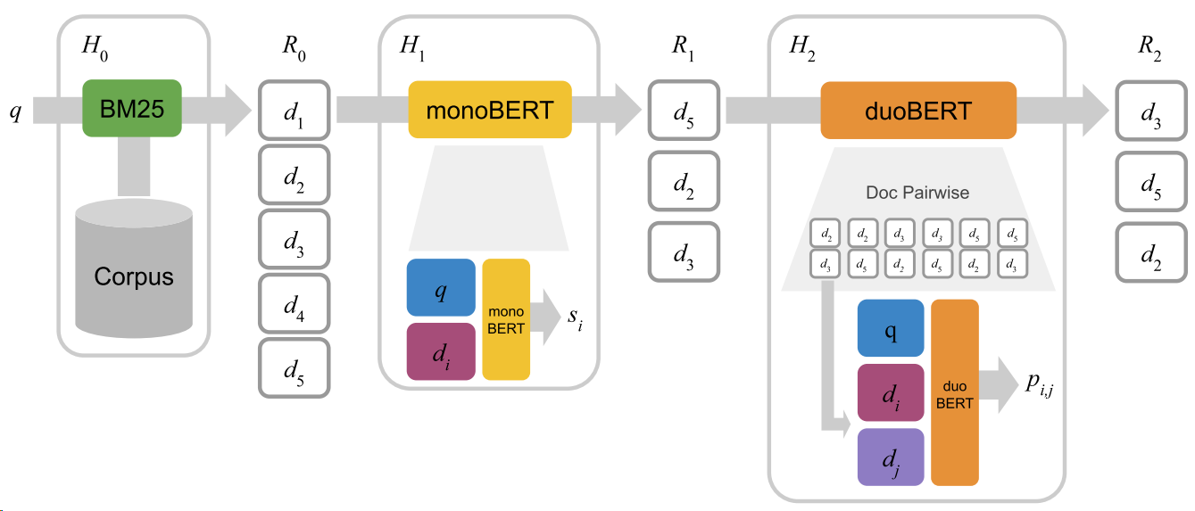
Fig. 24.6 Illustration of a three-stage retrieval-ranking architecture using BM25, monoBERT and duoBERT. Image from [NYCL19].#
With BERT variants of different ranking capability, we can construct a multi-stage ranking architecture to select a handful of most relevant document from a large collection of candidate documents given a query. Consider a typical architecture comprising a number of stages from \(H_0\) ot \(H_N\). \(H_0\) is a exact-term matching stage using from an inverted index. \(H_0\) stage take billion-scale document as input and output thousands of candidates \(R_0\). For stages from \(H_1\) to \(H_N\), each stage \(H_{n}\) receives a ranked list \(R_{n-1}\) of candidates from the previous stage and output candidate list \(R_n\). Typically \(|R_n| \ll |R_{n-1}|\) to enable efficient retrieval.
An example three-stage retrieval-ranking system is shown in Fig. 24.6. In the first stage \(H_{0}\), given a query \(q\), the top candidate documents \(R_{0}\) are retrieved using BM25. In the second stage \(H_{1}\), monoBERT produces a relevance score \(s_{i}\) for each pair of query \(q\) and candidate \(d_{i} \in R_{0}.\) The top candidates with respect to these relevance scores are passed to the last stage \(H_{2}\), in which duoBERT computes a relevance score \(p_{i, j}\) for each triple \(\left(q, d_{i}, d_{j}\right)\). The final list of candidates \(R_{2}\) is formed by re-ranking the candidates according to these scores .
Evaluation. Different multistage architecture configurations are evaluated using the MS MARCO dataset. We have following observations:
Using a single stage of BM25 yields the worst performance.
Adding an additional monoBERT significantly improve the performance over the single BM25 stage architecture.
Adding the third component duoBERT only yields a diminishing gain.
Further, the author found that employing the technique of Target Corpus Pre-training (TCP)\ gives additional performance gain. Specifically, the BERT backbone will undergo a two-phase pre-training. In the first phase, the model is pre-trained using the original setup, that is Wikipedia (2.5B words) and the Toronto Book corpus ( 0.8B words) for one million iterations. In the second phase, the model is further pre-trained on the MS MARCO corpus.
Method |
Dev |
Eval |
|---|---|---|
Anserini (BM25) |
18.7 |
19.0 |
+ monoBERT |
37.2 |
36.5 |
+ monoBERT + duoBERTMAX |
32.6 |
- |
+ monoBERT + duoBERTMIN |
37.9 |
- |
+ monoBERT + duoBERTSUM |
38.2 |
37.0 |
+ monoBERT + duoBERTBINARY |
38.3 |
- |
+ monoBERT + duoBERTSUM + TCP |
39.0 |
37.9 |
24.2.6. DC-BERT#
One way to improve the computational efficiency of cross-encoder is to employ bi-encoders for partial separate encoding and then employ an additional shallow module for cross encoding. One example is the architecture shown in Fig. 24.7, which is called DC-BERT and proposed in [NZG+20]. The overall architecture of DC-BERT consists of a dual-BERT component for decoupled encoding, a Transformer component for question-document interactions, and a binary classifier component for document relevance scoring.
The document encoder can be run offline to pre-encodes all documents and caches all term representations. During online inference, we only need to run the BERT query encodes online. Then the obtained contextual term representations are fed into high-layer Transformer interaction layer.
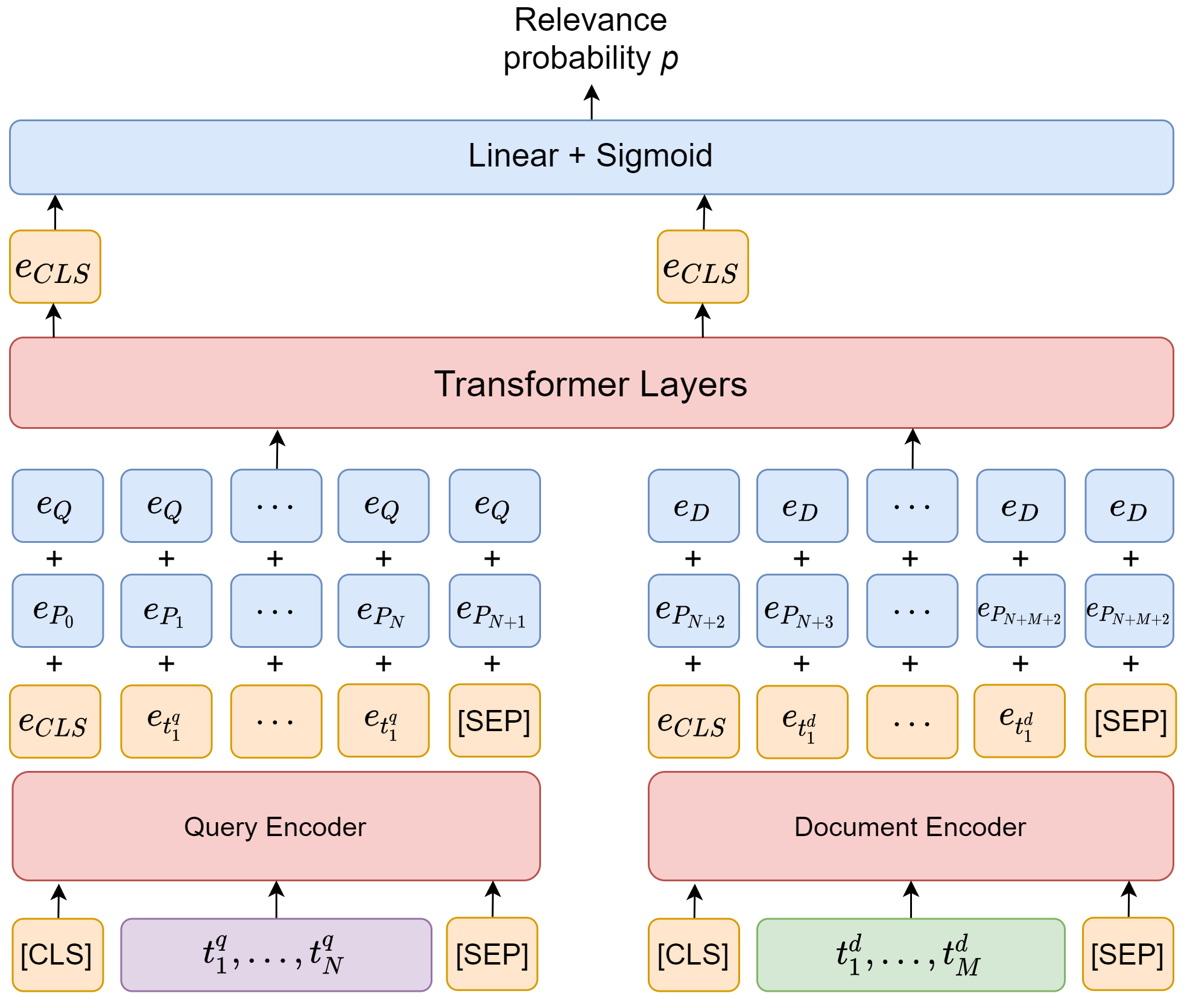
Fig. 24.7 The overall architecture of DC-BERT consists of a dual-BERT component for decoupled encoding, a Transformer component for question-document interactions, and a classifier component for document relevance scoring.#
Dual-BERT component. DC-BERT contains two pre-trained BERT models to independently encode the question and each retrieved document. During training, the parameters of both BERT models are fine-tuned to optimize the learning objective.
Transformer component. The dual-BERT components produce contextualized embeddings for both the query token sequence and the document token sequence. Then we add global position embeddings \(\mathbf{E}_{P_{i}} \in \mathbb{R}^{d}\) and segment embedding again to re-encode the position information and segment information (i.e., query vs document). Both the global position and segment embeddings are initialized from pre-trained BERT, and will be fine-tuned. The number of Transformer layers \(K\) is configurable to trade-off between the model capacity and efficiency. The Transformer layers are initialized by the last \(K\) layers of pre-trained BERT, and are fine-tuned during the training.
Classifier component. The two CLS token output from the Transformer layers will be fed into a linear binary classifier to predict whether the retrieved document is relevant to the query. Following previous work (Das et al., 2019; Htut et al., 2018; Lin et al., 2018), we employ paragraph-level distant supervision to gather labels for training the classifier, where a paragraph that contains the exact ground truth answer span is labeled as a positive example. We parameterize the binary classifier as a MLP layer on top of the Transformer layers:
where \(\left(q_{i}, d_{j}\right)\) is a pair of question and retrieved document, and \(o_{[C L S]}\) and \(o_{[C L S]}^{\prime}\) are the Transformer output encodings of the [CLS] token of the question and the document, respectively. The MLP parameters are updated by minimizing the cross-entropy loss.
DC-BERT uses one Transformer layer for question-document interactions. Quantized BERT is a 8bit-Integer model. DistilBERT is a compact BERT model with 2 Transformer layers.
We first compare the retriever speed. DC-BERT achieves over 10x speedup over the BERT-base retriever, which demonstrates the efficiency of this method. Quantized BERT has the same model architecture as BERT-base, leading to the minimal speedup. DistilBERT achieves about 6x speedup with only 2 Transformer layers, while BERT-base uses 12 Transformer layers.
With a 10x speedup, DC-BERT still achieves similar retrieval performance compared to BERT- base on both datasets. At the cost of little speedup, Quantized BERT also works well in ranking documents. DistilBERT performs significantly worse than BERT-base, which shows the limitation of the distilled BERT model.
Model |
SQuAD |
Natural Questions |
||
|---|---|---|---|---|
PTB@10 |
Speedup |
P@10 |
Speedup |
|
BERT-base |
71.5 |
1.0x |
65.0 |
1.0x |
Quantized BERT |
68.0 |
1.1x |
64.3 |
1.1x |
DistilBERT |
56.4 |
5.7x |
60.6 |
5.7x |
DC-BERT |
70.1 |
10.3x |
63.5 |
10.3x |
To further investigate the impact of our model architecture design, we compare the performance of DC-BERT and its variants, including 1) DC-BERT-Linear, which uses linear layers instead of Transformers for interaction; and 2) DC-BERT-LSTM, which uses LSTM and bi- linear layers for interactions following previous work (Min et al., 2018). We report the results in Table 3. Due to the simplistic architecture of the interaction layers, DC-BERT-Linear achieves the best speedup but has significant performance drop, while DC-BERT-LSTM achieves slightly worse performance and speedup than DC-BERT.
Retriever Model |
Retriever P@10 |
Retriever Speedup |
|---|---|---|
DC-BERT-Linear |
57.3 |
43.6x |
DC-BERT-LSTM |
61.5 |
8.2x |
DC-BERT |
63.5 |
10.3x |
24.2.7. Multi-Attribute and Multi-task Modeling#
We can extend cross-encoder to take into multiple-attributes from query side and document side, as well as generating multiple predictive outputs for different tasks [Fig. 24.8].
For example, query side attributes could include
Query text
Query’s language (produced by a cheapter language detection model)
User’s location and region
Other query side signals (e.g., key concept groups in the query, document signals from historical queries) Document side attributes could include
Organic contents with semantic markers (e.g., [T] for Title)
Other derived signals from documents (e.g., puesedo queries, historical queries, etc.) Other high level signals suitable late stage fusion
Document refreshness attribute (for intent to search latest news)
Document spamness attributes
After feature fusion (e.g., via concatination), we can separate MLP head for different tasks
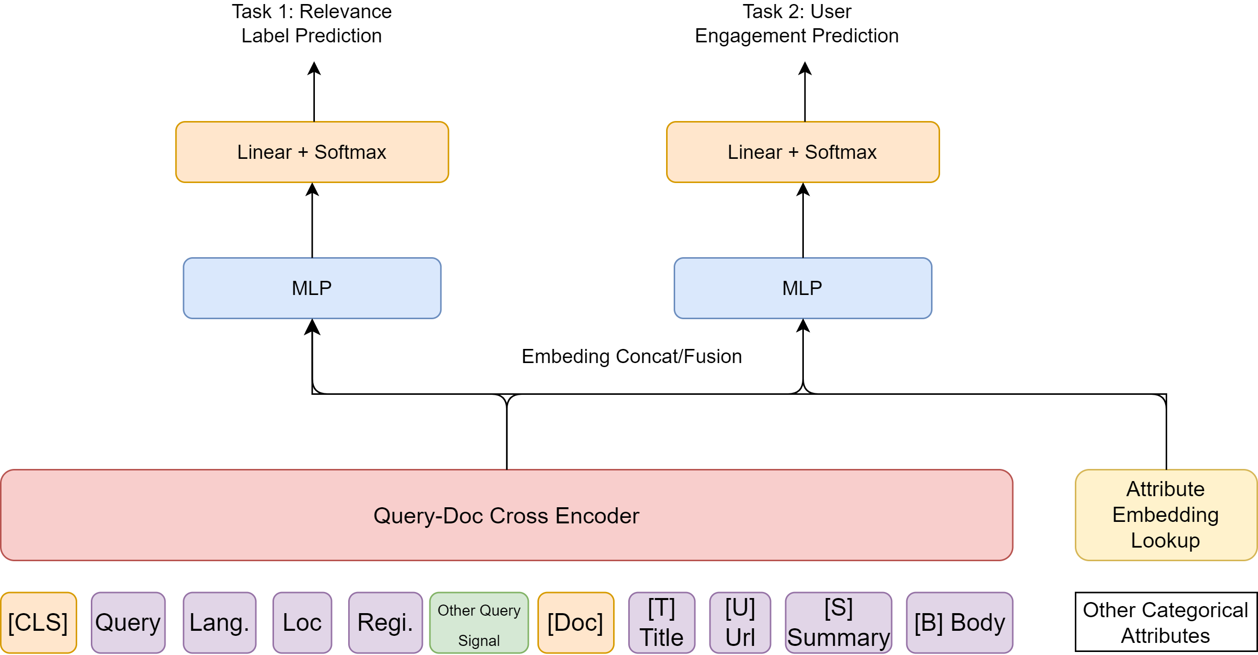
Fig. 24.8 An representative cross-encoder that is extended to take into account multiple-attributes from query side and document side. There are multiple outputs for multi-tasking.#
24.3. Multi-Vector Retrievers#
24.3.1. Introduction#
In classic representation-based learning for semantic retrieval [Classic Representation-based Learning], we use two encoders (i.e., bi-encoders) to separately encoder a query and a candidate document into two dense vectors in the embedding space, and then a score function, such as cosine similarity, to produce the final relevance score. In this paradigm, there is a single global, static representation for each query and each document. Specifically, the document’s embedding remain the same regardless of the document length, the content structure of document (e.g., multiple topics) and the variation of queries that are relevant to the document. It is very common that a document with hundreds of tokens might contain several distinct subtopics, some important semantic information might be easily missed or biased by each other when compressing a document into a dense vector. As such, this simple bi-encoder structure may cause serious information loss when used to encode documents. [^2]
On the other hand, cross-encoders based on BERT variants utilize multiple self-attention layers not only to extract contextualized features from queries and documents but also capture the interactions between them. Cross-encoders only produce intermediate representations that take a pair of query and document as the joint input. While BERT-based cross-encoders brought significant performance gain, they are computationally prohibitive and impractical for online inference.
In this section, we focus on different strategies [HSLW19, LETC21, TSJ+21] to encode documents by multi-vector representations, which enriches the single vector representation produced by a bi-encoder. With additional computational overhead, these strategies can gain much improvement of the encoding quality while retaining the fast retrieval strengths of Bi-encoder.
24.3.2. ColBERT#
24.3.2.1. Overview#
ColBERT [KZ20] is another example architecture that consists of an early separate encoding phase and a late interaction phase, as shown in Fig. 24.9. ColBERT employs a single BERT model for both query and document encoders but distinguish input sequences that correspond to queries and documents by prepending a special token [Q] to queries and another token [D] to documents.
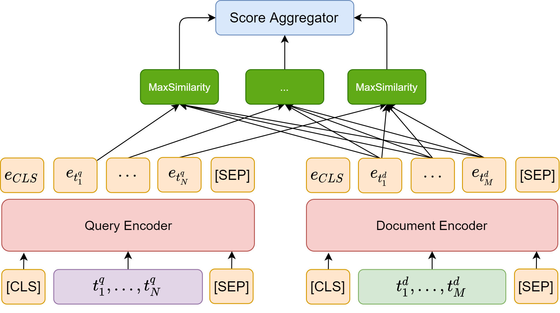
Fig. 24.9 The architecture of ColBERT, which consists of an early separate encoding phase and a late interaction phase.#
24.3.2.2. Encoding#
The query Encoder take query tokens as the input. Note that if a query is shorter than a pre-defined number \(N_q\), it will be padded with BERT’s special [mask] tokens up to length \(N_q\); otherwise, only the first \(N_q\) tokens will be kept. It is found that the mask token padding serves as some sort of query augmentation and brings perform gain. In additional, a [Q] token is placed right after BERT’s sequence start token [CLS]. The query encoder then computes a contextualized representation for the query tokens.
The document encoder has a very similar architecture. A [D] token is placed right after BERT’s sequence start token [CLS]. Note that after passing through the encoder, embeddings correponding to punctuation symbols are filtered out.
Given BERT’s representation of each token, an additional linear layer with no activation is used to reduce the dimensionality reduction. The reduced dimensionality \(m\) is set much smaller than BERT’s fixed hidden dimension.
Finally, given \(q= q_{1} \ldots q_{l}\) and \(d=d_{1} \ldots d_{n}\), an additional CNN layer is used to allow each embedding vector to interact with its neighbor, yielding the bags of embeddings \(E_{q}\) and \(E_{d}\) in the following manner.
Here # refers to the [Mask] tokens and \(\operatorname{Normalize}\) denotes \(L_2\) length normalization.
24.3.2.3. Late Interaction#
In the late interaction phase, every query embedding interacts with all document embeddings via a MaxSimilarity operator, which computes maximum similarity (e.g., cosine similarity), and the scalar outputs of these operators are summed across query terms.
Formally, the final similarity score between the \(q\) and \(d\) is given by
where \(I_q = \{1,...,l\}\), \(I_d = \{1, ..., n\}\) are the index sets for query token embeddings and document token embeddings, respectively. ColBERT is differentiable end-to-end and we can fine-tune the BERT encoders and train from scratch the additional parameters (i.e., the linear layer and the \([Q]\) and \([D]\) markers’ embeddings). Notice that the final aggregation interaction mechanism has no trainable parameters.
24.3.2.4. Retrieval & Re-ranking#
The retrieval and re-ranking using ColBert consists of three steps:
Token retrieving doc token candidates from index via query token embedding, with doc token’s source canddiate being the doc candidates,
Gathering all token vectors for doc candidates,
Scoring the candidate documents using all its token embeddings
The first retrieval step further consists of two-steps:
each query token (out of \(N_q\) tokens) first retrieves top \(k'\) (e.g., \(k'=k/2\)) document IDs using approximate nearest neighbor (ANN) search. See more in Approximate Nearest Neighbor Search.
Merge \(N_q \times k'\) documents ID to get \(K\) unique documents as the retrieval result.
After retrieving top-\(k\) documents given a query \(q\), the next step is score these \(k\) documents as the **re-ranking **step. Specifically, with a query \(q\) represented by a bag contextualized embeddings \(E_q\) (a 2D matrix) and we further gather the document representations into a 3-dimensional tensor \(D\) consisting of \(k\) document matrices. For each query and document pair, we compute its score according to (24.1).
24.3.2.5. Evaluation#
The retrieval performance of ColBERT is evaluated on MS MARCO dataset. Compared with traditional exact term matching retrieval BM25, ColBERT has shortcomings in terms of latency but MRR is significantly better.
Method |
MRR@10(Dev) |
MRR@10 (Local Eval) |
Latency (ms) |
Recall@50 |
|---|---|---|---|---|
BM25 (Anserini) |
18.7 |
19.5 |
62 |
59.2 |
doc2query |
21.5 |
22.8 |
85 |
64.4 |
DeepCT |
24.3 |
- |
62 (est.) |
69[2] |
docTTTTTquery |
27.7 |
28.4 |
87 |
75.6 |
ColBERT L2 (BM25 + re-rank) |
34.8 |
36.4 |
- |
75.3 |
ColBERTL2 (retrieval & re-rank) |
36.0 |
36.7 |
458 |
82.9 |
Similarly, we can evaluate ColBERT’s re-ranking performance against some strong baselines, such as BERT cross encoders [NC19, NYCL19]. ColBERT has demonstrated significant benefits in reducing latency with little cost of re-ranking performance.
Method |
MRR@10 (Dev) |
MRR@10 (Eval) |
Re-ranking Latency (ms) |
|---|---|---|---|
BM25 (official) |
16.7 |
16.5 |
- |
KNRM |
19.8 |
19.8 |
3 |
Duet |
24.3 |
24.5 |
22 |
fastText+ConvKNRM |
29.0 |
27.7 |
28 |
BERT base |
34.7 |
- |
10,700 |
BERT large |
36.5 |
35.9 |
32,900 |
ColBERT (over BERT base) |
34.9 |
34.9 |
61 |
24.3.3. Semantic Clusters As Pseudo Query Embeddings#
The primary limitation of Bi-encoder is information loss when we condense the document into a query agnostic dense vector representation. Authors in [TSJ+21] proposed the idea of representing a document by its semantic salient fragments [Fig. 24.10]. These semantic fragments can be modeled by token embedding vector clusters in the embedding space. By performing clustering algorithms (e.g., k-means) on token embeddings, the generated centroids can be used as a document’s multi-vector presentation. Another interpretation is that these centroids can be viewed as multiple potential queries corresponding to the input document; as such, we can call them pseudo query embeddings.
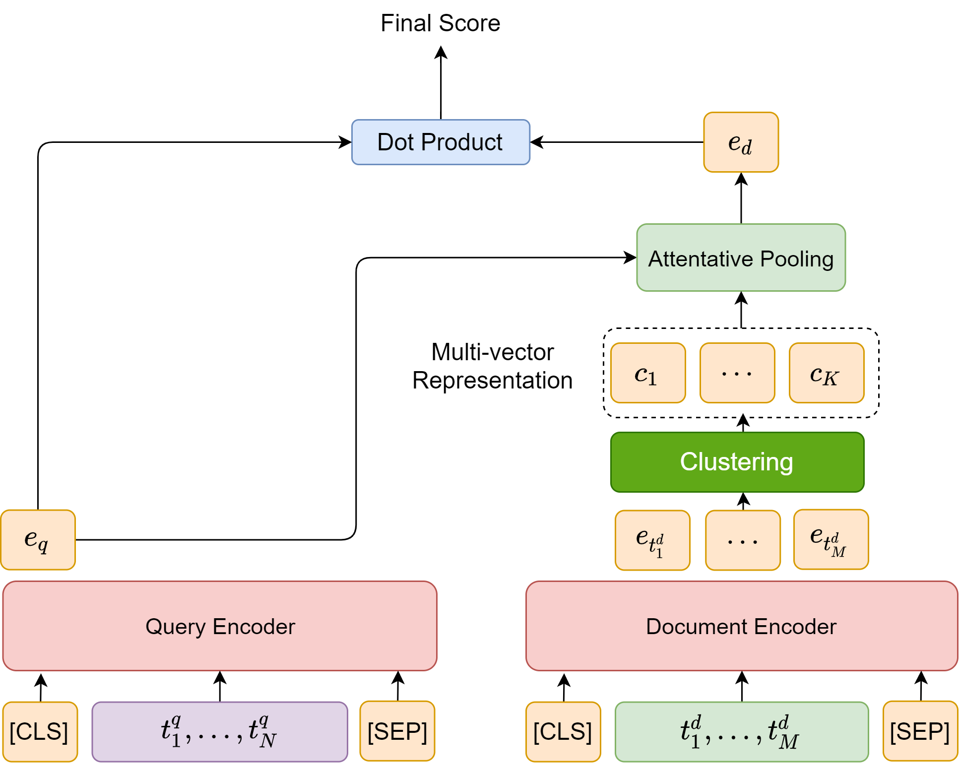
Fig. 24.10 Deriving semantic clusters by clustering token-level embedding vectors. Semantic cluster centroids are used as multi-vector document representation, or as pseudo query embeddings. The final relevance score between a query and a document is computed using attententive pooling of centroid cluster and doc product.#
There are a couple of steps to calculate the final relevance score between a query and a document. First, we encode the query \(q\) into a dense vector \(e_q\) (via the CLS token embedding) and the document \(d\) into multiple vectors via token level encoding and clustering \(c_1,...,c_K\). Second, the query-conditional document representation \(e_d\) is obtained by attending to the centroids using \(e_q\) as the key. Finally, we can compute the similarity score via dot product between \(e_q\) and \(e_d\).
In summary, we have
In practice, we can save the centroid embeddings in memory and retrieve them using the real queries.
24.3.4. Token-level Representation and Retrieval (ColBert)#
To enrich the representations of the documents produced by Bi-encoder, some researchers extend the original Bi-encoder by employing more delicate structures like later-interaction.
ColBERT [Section 24.3.2] can be viewed a token-level multi-vector representation encoder for both queries and documents. Token-level representations for documents can be pre-computed offline. During online inference, late interactions of the query’s multi-vectors representation and the document’s multi-vectors representation are used to improve the robustness of dense retrieval, as compared to inner products of single-vector representations. Specifically,
Formally, given \(q= q_{1} \ldots q_{l}\) and \(d=d_{1} \ldots d_{n}\) and their token level embeddings \(\{E_{q_1},\ldots E_{q_l}\}\) and \(\{E_{d_1},...,E_{d_n}\}\) and the final similarity score between the \(q\) and \(d\) is given by
where \(I_q = \{1,...,l\}\), \(I_d = \{1, ..., n\}\) are the index sets for query token embeddings and document token embeddings, respectively.
While this method has shown signficant improvement over bi-encoder methods, it has a main disadvantage of high storage requirements. For example, ColBERT requires storing all the WordPiece token vectors of each text in the corpus.
24.3.5. Colbert v2#
24.4. Ranker Training#
24.4.1. Overview#
Unlike in classification or regression, the main goal of a ranker[AWB+19] is not to assign a label or a value to individual items, but to produce an ordering of the items in that list in such a way that the utility of the entire list is maximized.
In other words, in ranking we are more concerned with the relative ordering items, instead of predicting the numerical value or label of an individual item.
Pointwise ranking transforms the ranking problem into a regression problem. Given a certain Query, ranking amounts to
Predict the relevance score between the document to the query
Order the document list based on its relevance score with the query.
Pairwise Ranking[Bur10], instead of predicting the absolute relevance, learns to predict the relative order of documents. This method is particularly useful in scenarios where the absolute relevance scores are less important than the relative ordering of items,
Listwise ranking [CQL+07] considers the entire list of items simultaneously when training a ranking model. Unlike pairwise or pointwise methods, listwise ranking directly optimizes ranking metrics such as NDCG or MAP, which better aligns the training objective with the evaluation criteria used in information retrieval tasks. This approach can capture more complex relationships between items in a list and often leads to better performance in real-world ranking scenarios, though it may be computationally more expensive than other ranking methods.
24.4.2. Training Data#
In a typical model learning setting, we construct training data from user search log, which contains queries issued by users and the documents they clicked after issuing the query. The basic assumption is that a query and a document are relevant if the user clicked the document.
Model learning in information retrieval typically falls into the category of contrastive learning. The query and the clicked document form a positive example; the query and irrelevant documents form negative examples. For retrieval problems, it is often the case that positive examples are available explicitly, while negative examples are unknown and need to be selected from an extremely large pool. The strategy of selecting negative examples plays an important role in determining quality of the encoders. In the most simple case, we randomly select unclicked documents as irrelevant document, or negative example. We defer the discussion of advanced negative example selecting strategy to Section 24.5.
When there is a shortage of annotation data or click behavior data, we can also leverage weakly supervised data for training [DZS+17, HG19, NSN18, RSL+21]. In the weakly supervised data, labels or signals are obtained from an unsupervised ranking model, such as BM25. For example, given a query, relevance scores for all documents can be computed efficiently using BM25. Documents with highest scores can be used as positive examples and documents with lower scores can be used as negatives or hard negatives.
24.4.3. Pointwise Ranking#
24.4.3.1. Pointwise Regression Objective#
The idea of pointwise regression objective is to model the numerical relevance score for a given query-document. During inference time, the relevance scores between a set of candidates and a given query can be predicted and ranked.
During training, given a set of query-document pairs \(\left(q_{i}, d_{i, j}\right)\) and their corresponding relevance score \(y_{i, j} \in [0, 1]\) and their prediction \(f(q_i,d_{i,j})\). A pointwise regression objective tries to optimize a model to predict the relevance score via minimization
Using a regression objective offer flexible for the user to model different levels of relevance between queries and documents. However, such flexibility also comes with** a requirement that the target relevance score should be accurate in absolute scale.** While human annotated data might provide absolute relevance score, human annotation data is expensive and small scale. On the other hand, absolute relevance scores that are approximated by click data can be noisy and less optimal for regression objective. To make** training robust to label noises**, one can consider Pairwise ranking objectives. This particularly important in weak supervision scenario with noisy label. Using the ranking objective alleviates this issue by forcing the model to learn a preference function rather than reproduce absolute scores.
24.4.3.2. Pointwise Ranking Objective#
The idea of pointwise ranking objective is to simplify a ranking problem to a binary classification problem. Specifically, given a set of query-document pairs \(\left(q_{i}, d_{i, j}\right)\) and their corresponding relevance label \(y_{i, j} \in \{0, 1\}\), where 0 denotes irrelevant and 1 denotes relevant. A pointwise learning objective tries to optimize a model to predict the relevance label.
A commonly used pointwise loss functions is the binary Cross Entropy loss:
where \(p\left(q_{i}, d{i, j}\right)\) is the predicted probability of document \(d_{i,j}\) being relevant to query \(q_i\).
The advantages of pointwise ranking objectives are two-fold. First, pointwise ranking objectives are computed based on each query-document pair \(\left(q_{i}, d_{i, j}\right)\) separately, which makes it simple and easy to scale. Second, the outputs of neural models learned with pointwise loss functions often have real meanings and value in practice. For instance, in sponsored search, the predicted the relevance probability can be used in ad bidding, which is more important than creating a good result list in some application scenarios.
In general, however, pointwise ranking objectives are considered to be less effective in ranking tasks. Because pointwise loss functions consider no document preference or order information, they do not guarantee to produce the best ranking list when the model loss reaches the global minimum. Therefore, better ranking paradigms that directly optimize document ranking based on pairwise loss functions and even listwise loss functions.
24.4.4. Pairwise Ranking via Triplet Loss#
Pointwise ranking loss aims to optimize the model to directly predict relevance between query and documents on absolute score. From embedding optimization perspective, it train the neural query/document encoders to produce similar embedding vectors for a query and its relevant document and dissimilar embedding vectors for a query and its irrelevant documents.
On the other hand, pairwise ranking objectives focus on optimizing the relative preferences between documents rather than predicting their relevance labels. In contrast to pointwise methods where the final ranking loss is the sum of loss on each document, pairwise loss functions are computed based on the different combination of document pairs.
One of the most common pairwise ranking loss function is the triplet loss. Let \(\mathcal{D}=\left\{\left\langle q_{i}, d_{i}^{+}, d_{i}^{-}\right\rangle\right\}_{i=1}^{m}\) be the training data organized into \(m\) triplets. Each triplet contains one query \(q_{i}\) and one relevant document \(d_{i}^{+}\), along with one irrelevant (negative) documents \(d_{i}^{-}\). Negative documents are typically randomly sampled from a large corpus or are strategically constructed [Section 24.5]. Visualization of the learning process in the embedding space is shown in Fig. 24.11. Triplet loss helps guide the encoder networks to pull relevant query and document closer and push irrelevant query and document away.
The loss function is given by
where \(\operatorname{Sim}(q, d)\) is the similarity score produced by the network between the query and the document and \(m\) is a hyper-parameter adjusting the margin. Clearly, if we would like to make \(L\) small, we need to make \(\operatorname{Sim}(q_i, d_i^+) - \operatorname{Sim}(q_i, d^-_i) > m\). Commonly used \(\operatorname{Sim}\) functions include dot product or Cosine similarity (i.e., length-normalized dot product), which are related to distance calculation in the Euclidean space and hyperspherical surface.
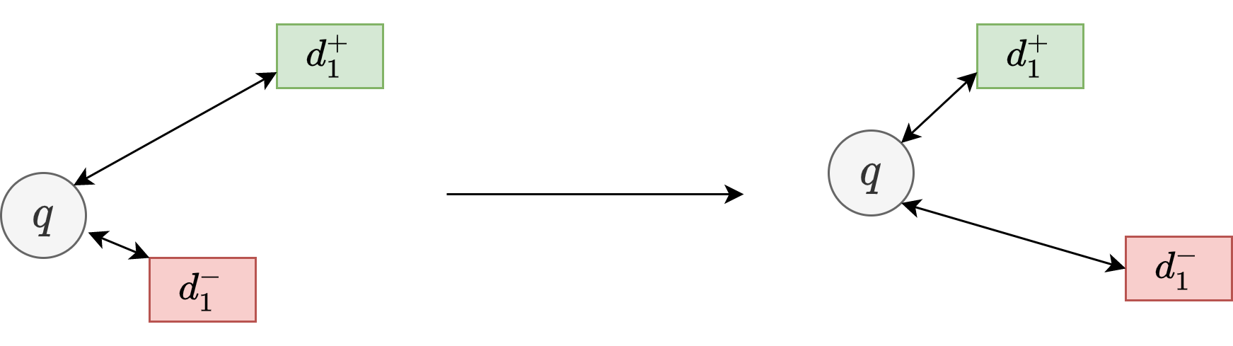
Fig. 24.11 The illustration of the learning process (in the embedding space) using triplet loss.#
Triplet loss can also operating in the angular space
As illustrated in Figure 1, the training objective is to score the positive example \(d^{+}\)by at least the margin \(\mu\) higher than the negative one \(d^{-}\). As part of our loss function, we use the triplet margin objective:
24.4.5. N-pair Contrastive Loss#
24.4.5.1. N-pair Loss#
Triplet loss optimize the neural by encouraging positive pair \((q_i, d^+_i)\) to be more similar than its negative pair \((q_i, d^+_i)\). One improvement is to encourage \(q_i\) to be more similar \(d^+_i\) compared to \(n\) negative examples \( d_{i, 1}^{-}, \cdots, d_{i, n}^{-}\), instead of just one negative example. This is known as N-pair loss [Soh16], and it is typically more robust than triplet loss.
Let \(\mathcal{D}=\left\{\left\langle q_{i}, d_{i}^{+}, D_i^-\right\rangle\right\}_{i=1}^{m}\), where \(D_i^- = \{d_{i, 1}^{-}, \cdots, d_{i, n}^{-}\}\) are a set of negative examples (i.e., irrelevant document) with respect to query \(q_i\), be the training data that consists of \(m\) examples. Each example contains one query \(q_{i}\) and one relevant document \(d_{i}^{+}\), along with \(n\) irrelevant (negative) documents \(d_{i, j}^{-}\). The \(n\) negative documents are typically randomly sampled from a large corpus or are strategically constructed [Section 24.5].
Visualization of the learning process in the embedding space is shown in Fig. 24.12. Like triplet loss, N-pair loss helps guide the encoder networks to pull relevant query and document closer and push irrelevant query and document away. Besides that, when there are are negatives are involved in the N-pair loss, their repelling to each other appears to help the learning of generating more uniform embeddings[WI20].
The loss function is given by
where \(\operatorname{Sim}(e_q, e_d)\) is the similarity score function taking query embedding \(e_q\) and document embedding \(e_d\) as the input.
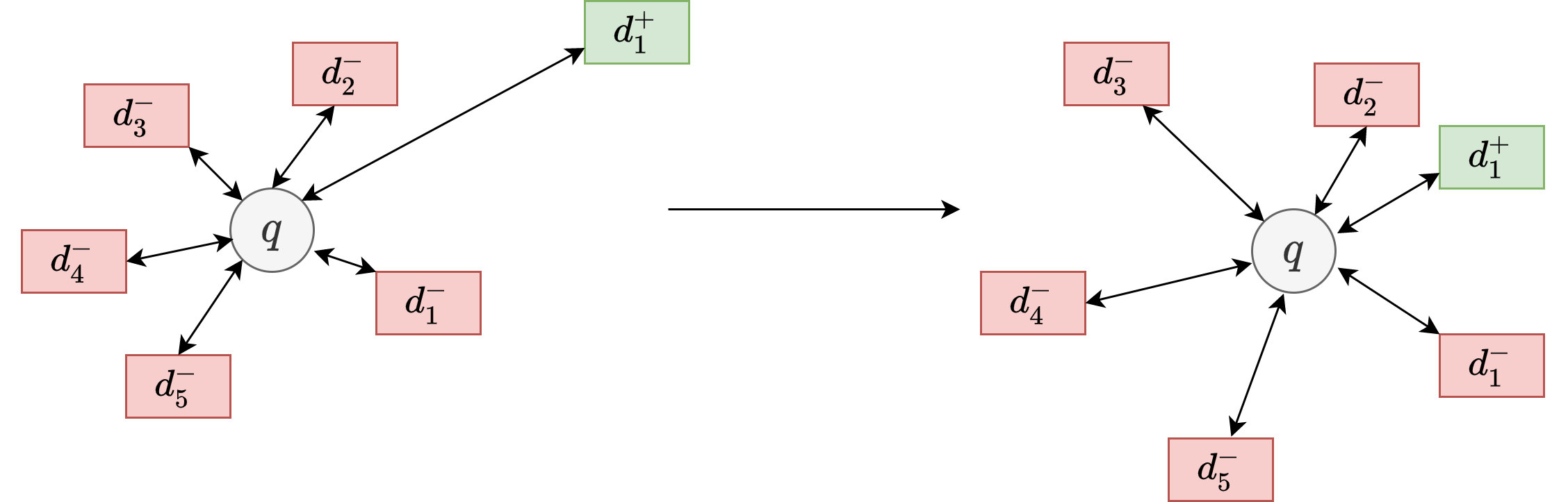
Fig. 24.12 The illustration of the learning process (in the embedding space) using N-pair loss.#
Remark 24.1 (Probability interprete of Log Softmax loss)
From langugae modeling perspetive [HARS+17], given a query \(q\), let \(d\) be the response to \(q\). The likelihood of observing \(d^+\) given \(q\) is by conditional probability
Further,
We approximate the joint probability by \(P(d, q) \propto \exp(\operatorname{Sim}(e_q, e_d))\)
We approximate \(\sum_d P(d, q)\) by the positve and sampled negatives via \(\sum_{d \in \{d^+,D^-\}} \exp(\operatorname{Sim}(e_q, e_d))\)
Then we have
The goal is to maximize the likelihood of \(P(d^+ | q)\) can be then translated to minimizing \(-\log P(d^+|q)\), which leads to (24.2).
24.4.5.2. N-pair Dual Loss#
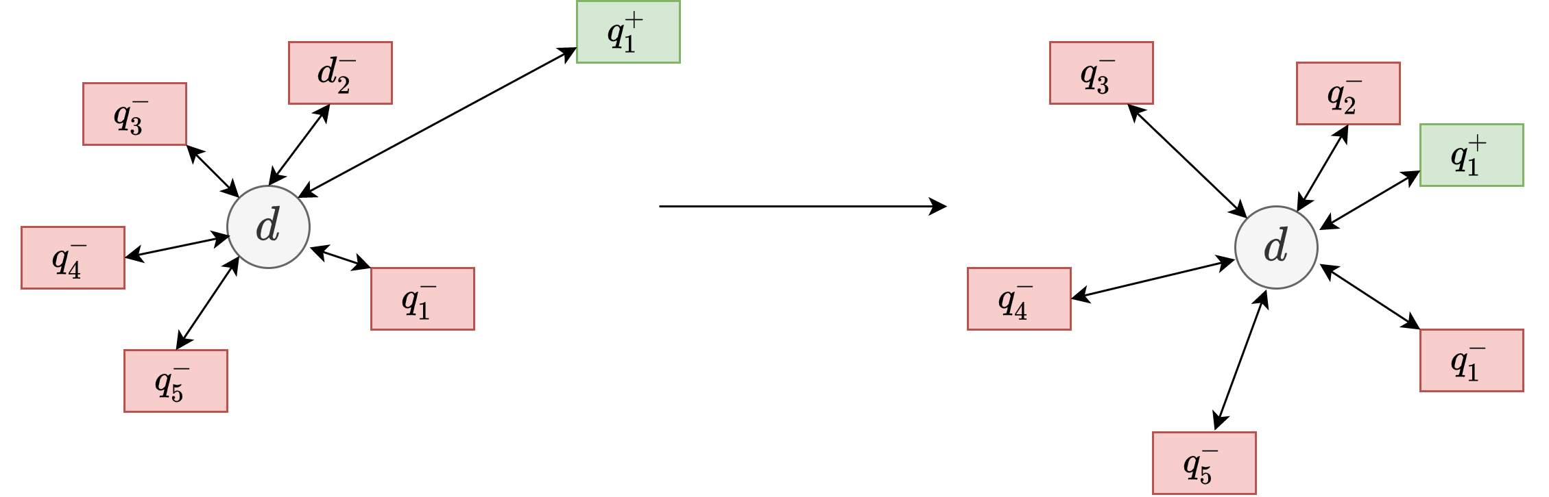
Fig. 24.13 The illustration of the learning process (in the embedding space) using N-pair dual loss.#
The N-pair loss uses query as the anchor to adjust the distribution of document vectors in the embedding space. Authors in [LLXL21] proposed that document can also be as the anchor to adjust the distribution of query vectors in the embedding space. This leads to loss functions consisting of two parts
where \(\operatorname{Sim}(e_q, e_d)\) is a symmetric similarity score function for the query and the document embedding vectors, \(L_{prime}\) is the N-pair loss, and \(L_{dual}\) is the N-pair dual loss.
To compute dual loss, we need to prepare training data \(\mathcal{D}_{dual}=\left\{\left\langle d_{i}, q_{i}^{+}, Q_i^-\right\rangle\right\}_{i=1}^{m}\), where \(Q_i^- = \{q_{i, 1}^{-}, \cdots, q_{i, n}^{-}\}\) are a set of negative queries examples (i.e., irrelevant query) with respect to document \(d_i\). Each example contains one document \(d_{i}\) and one relevant query \(d_{i}^{+}\), along with \(n\) irrelevant (negative) queries \(q_{i, j}^{-}\).
24.4.5.3. Doc-Doc N-pair Loss#
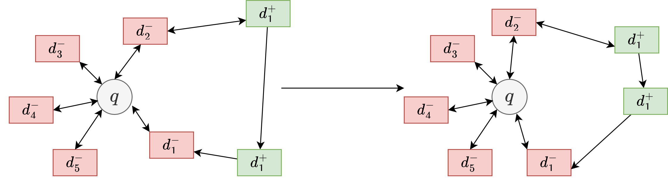
Fig. 24.14 The illustration of the learning process (in the embedding space) using Doc-Doc N-pair loss.#
Besiding use above prime and dual loss to capture robust query doc relationship, we can also improve robustness of document representation by considering doc-doc relations. Particularly,
When there are multiple positive documents associated with the same query, we use loss function encourage their representation embedding to stay close.
For positive and negative documents associated with the same query, we use loss function encourage their representation embedding to stay far apart.
The loss function is given by
where \(\operatorname{Sim}(e_{d_1}, e_{d_2})\) is the similarity score function taking document embeddings \(e_{d_1}\) and \(e_{d_2}\) as the input.
24.4.6. Listwise Ranking#
Although the pairwise approach offers advantages, it ignores the fact that ranking is a prediction task on list of objects. [CQL+07]
In training, a set of queries \(Q=\left\{q^{(1)}, q^{(2)}, \cdots, q^{(m)}\right\}\) is given. Each query \(q^{(i)}\) is associated with a list of documents \(d^{(i)}=\left(d_1^{(i)}, d_2^{(i)}, \cdots, d_{n^{(i)}}^{(i)}\right)\), where \(d_j^{(i)}\) denotes the \(j\)-th document and \(n^{(i)}\) denotes the sizes of \(d^{(i)}\). Furthermore, each list of documents \(d^{(i)}\) is associated with a list of judgments (scores) \(y^{(i)}=\left(y_1^{(i)}, y_2^{(i)}, \cdots, y_{n^{(i)}}^{(i)}\right)\) where \(y_j^{(i)}\) denotes the judgment on document \(d_j^{(i)}\) with respect to query \(q^{(i)}\).
We then create a ranking function \(f\); for each feature vector \(x_j^{(i)}\) (corresponding to document \(d_j^{(i)}\) ) it outputs a score \(f\left(x_j^{(i)}\right)\). For the list of feature vectors \(x^{(i)}\) we obtain a list of scores \(z^{(i)}=\left(f\left(x_1^{(i)}\right), \cdots, f\left(x_{n^{(i)}}^{(i)}\right)\right)\). The objective of learning is formalized as minimization of the total losses with respect to the training data.
where \(L\) is a listwise loss function.
One can construct the comparison of two lists by comparing the top-one probability of each document, which is defined as
where \(s_j\) is the score of object \(j, j=1,2, \ldots, n\) and \(\phi\) is an increasing and strictly positive function.
There are two important properties derived from the top-one probability definition:
Forming probability - top one probabilities \(P_s(j), j=1,2, \ldots, n\) forms a probability distribution over the set of \(n\) objects.
Preserving order - given any two objects \(j\) and \(k\), if \(s_j>s_k, j \neq\) \(k, j, k=1,2, \ldots, n\), then \(P_s(j)>P_s(k)\).
Usually, one can define \(\phi\) as an exponential function. Then the top one probability is give by
With the use of top one probability, we can use Cross Entropy as the listwise loss function,
which aims to bring the predicted top-one probabilities to the labeled top-one probabilities.
Remark 24.2
The major difference in listwise loss and the pairwise loss is that the former uses document lists as instances while the latter uses document pairs as instances; When there are only two documents for each query, i.e., the listwise loss function becomes equivalent to the pairwise loss function in RankNet.
The time complexity of computing pairwise loss is of order \(O\left(n^2\right)\) where \(n\) denotes number of documents per query. In contrast the time complexity of computing listwise loss is only of order \(O\left(n\right)\), which allows listwise ranking loss to be more efficient.
24.5. Training Data Sampling Strategies#
24.5.1. Principles#
From the ranking perspective, both retrieval and re-ranking requires the generation of some order on the input samples. For example, given a query \(q\) and a set of candidate documents \((d_1,...,d_N)\). We need the model to produce an order list \(d_2 \succ d_3 ... \succ d_k\) according to their relevance to the query.
To train a model to produce the expected results during inference, we should ensure the training data distribution to matched with the inference time data distribution. Particularly, the inference time the candidate document distribution and ranking granularity differ vastly for retrieval tasks and re-ranking tasks [Fig. 24.15]. Specifically,
For the retrieval task, we typically need to identify top \(k (k=1000-10000)\) relevant documents from the entire document corpus. This is achieved by ranking all documents in the corpus with respect to the relevance of the query.
For the re-ranking task, we need to identify the top \(k (k=10)\) most relevant documents from the relevant documents generated by the retrieval task.
Clearly, features most useful in the retrieval task (i.e., distinguish relevant from irrelevant) are often not the same as the features most useful in re-ranking task (i.e., distinguish most relevant from less relevant). Therefore, the training samples for retrieval and re-ranking need to be constructed differently.
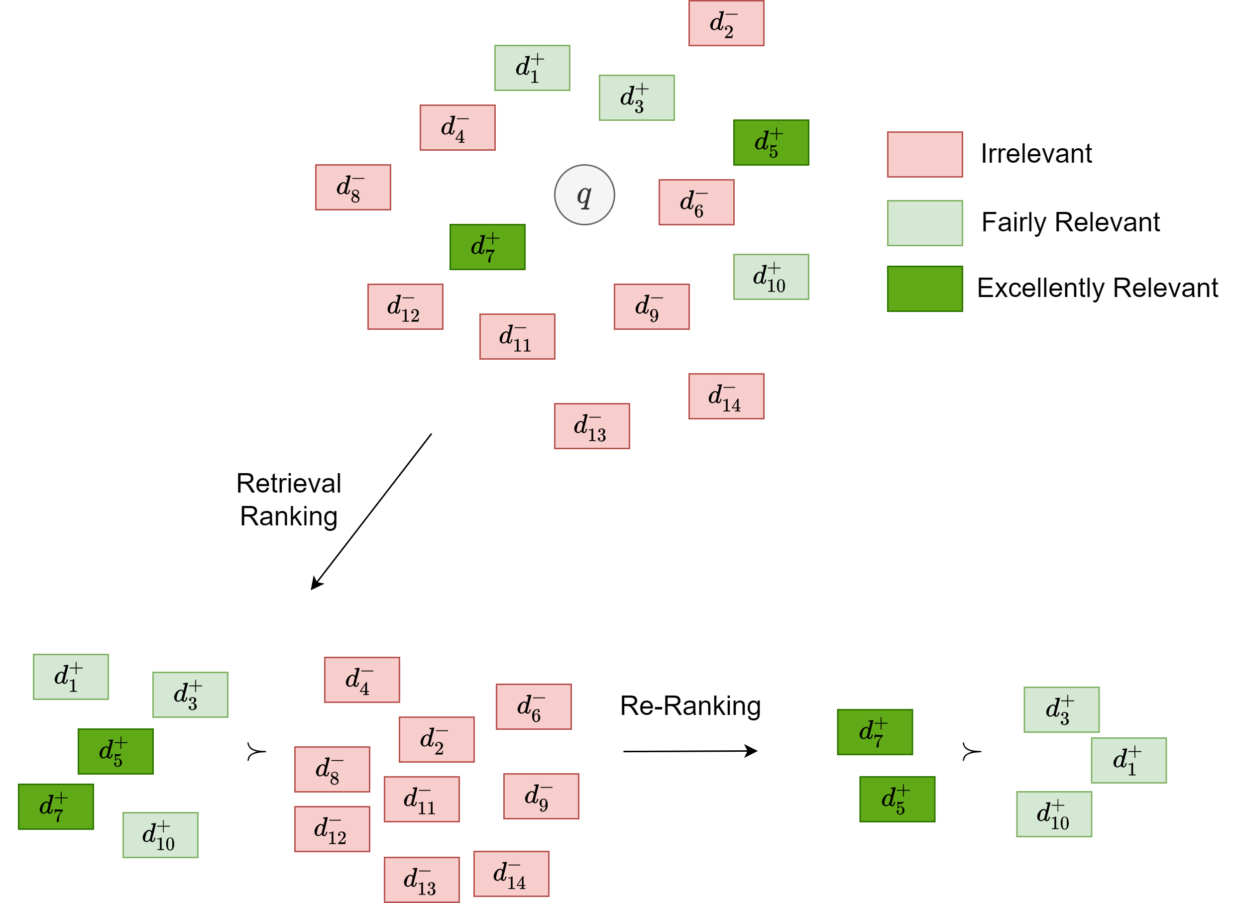
Fig. 24.15 Retrieval tasks and re-ranking tasks are faced with different the candidate document distribution and ranking granularity.#
Constructing the proper training data distribution is more challenging to retrieval stage than the re-ranking stage. In re-ranking stage, data in the training and inference phases are both the documents from previous retrieval stages. In the retrieval stage, we need to construct training examples in a mini-batch fashion in a way that each batch approximates the distribution in the inference phase as close as possible.
This section will mainly focus on constructing training examples for retrieval model training in an efficient and effective way. Since the number of negative examples (i.e., irrelevant documents) significantly outnumber the number of positive examples. Constructing training examples particularly boil down to constructing proper negative examples.
24.5.2. Negative Sampling Methods I: Heuristic Methods#
24.5.2.1. Random Negatives and In-batch Negatives#
Random negative sampling is the most basic negative sampling algorithm. The algorithm uniformly sample documents from the corpus and treat it as a negative. Clearly, random negatives can generate negatives that are too easy for the model. For example, a negative document that is topically different from the query. These easy negatives lower the learning efficiency, that is, each batch produces limited information gain to update the model. Still, random negatives are widely used because of its simplicity.
In practice, random negatives are implemented as in-batch negatives. In the contrastive learning framework with N-pair loss [Section 24.4.5.1], we construct a mini-batch of query-doc examples like \(\{(q_1, d_1^+, d_{1,1}^-, d_{1,M}^-), ..., (q_N, d_N^+, d_{N,1}^-, d_{N,M}^M)\}\), Naively implementing N-pair loss would increase computational cost from constructing sufficient negative documents corresponding to each query. In-batch negatives[KOuguzM+20] is trick to reuse positive documents associated with other queries as extra negatives [Fig. 24.16]. The critical assumption here is that queries in a mini-batch are vastly different semantically, and positive documents from other queries would be confidently used as negatives. The assumption is largely true since each mini-batch is randomly sampled from the set of all training queries, in-batch negative document are usually true negative although they might not be hard negatives.
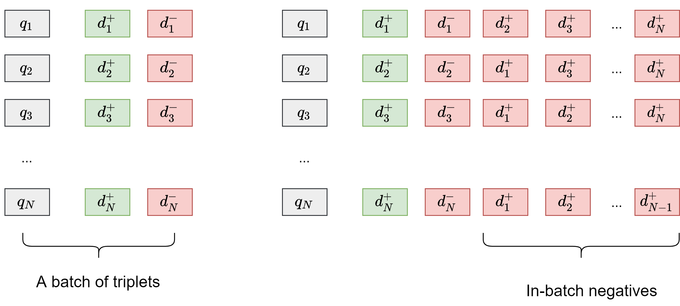
Fig. 24.16 The illustration of using in-batch negatives in contrastive learning.#
Specifically, assume that we have \(N\) queries in a mini-batch and each one is associated with a relevant positive document. By using positive document of other queries, each query will have an additional \(N - 1\) negatives.
Formally, we can define our batch-wise loss function as follows:
where \(l\left(q_{i}, d_{i}^{+}, d_{j}^{-}\right)\) is the loss function for a triplet.
In-batch negative offers an efficient implementation for random negatives. Another way to mitigate the inefficient learning issue is simply use large batch size (>4,000) [Cross-Batch Large-Scale Negatives].
24.5.2.2. Popularity-based Negative Sampling#
Popularity-based negative sampling use document popularity as the sampling weight to sample negative documents. The popularity of a document can be defined as some combination of click, dwell time, quality, etc. Compared to random negative sampling, this algorithm replaces the uniform distribution with a popularity-based sampling distribution, which can be pre-computed offline.
The major rationale of using popularity-based negative examples is to improve representation learning. Popular negative documents represent a harder negative compared to a unpopular negative since they tend to have to a higher chance of being more relevant; that is, lying closer to query in the embedding space. If the model is trained to distinguish these harder cases, the over learned representations will be likely improved.
Popularity-based negative sampling is also used in word2vec training [MSC+13]. For example, the probability to sample a word \(w_i\) is given by:
where \(f(w)\) is the frequency of word \(w\). This equation, compared to linear popularity, has the tendency to increase the probability for less frequent words and decrease the probability for more frequent words.
24.5.2.3. Topic-aware Negative Sampling#
In-batch random negatives would often consist of topically-different documents, leaving little information gain for the training. To improve the information gain from a single random batch, we can constrain the queries and their relevant document are drawn from a similar topic[HofstatterLY+21].
The procedures are
Cluster queries using query embeddings produced by basic query encoder.
Sample queries and their relevant documents from a randomly picked cluster. A relevant document of a query form the negative of the other query.
Since queries are topically similar, the formed in-batch negatives are harder examples than randomly formed in-batch negative, therefore delivering more information gain each batch.
Note that here we group queries into clusters by their embedding similarity, which allows grouping queries without lexical overlap. We can also consider lexical similarity between queries as additional signals to predict query similarity.
24.5.3. Negative Sampling Methods II: Model-based Methods#
24.5.3.1. Static Hard Negative Examples#
Deep model improves the encoded representation of queries and documents by contrastive learning, in which the model learns to distinguish positive examples and negative examples. A simple random sampling strategy tend to produce a large quantity of easy negative examples since easy negative examples make up the majority of negative examples. Here by easy negative examples, we mean a document that can be easily judged to be irrelevant to the query. For example, the document and the query are in completely different topics.
The model learning from easy negative example can quickly plateau since easy negative examples produces vanishing gradients to update the model. An improvement strategy is to supply additional hard negatives with randomly sampled negatives. In the simplest case, hard negatives can be selected based on a traditional BM25model [KOuguzM+20, NC19] or other efficient dense retriever: hard negatives are those have a high relevant score to the query but they are not relevant.
As illustrated in Fig. 24.17, a model trained only with easy negatives can fail to distinguish fairly relevant documents from irrelevant examples; on the other hand, a model trained with some hard negatives can learn better representations:
Positive document embeddings are more aligned [WI20]; that is, they are lying closer with respect to each other.
Fairly relevant and irrelevant documents are more separated in the embedding space and thus a better decision boundary for relevant and irrelevant documents.

Fig. 24.17 Illustration of importance of negative hard examples, which helps learning better representations to distinguish irrelevant and fairly relevant documents.#
In generating these negative examples, the negative-generation model (e.g., BM25) and the model under training are de-coupled; that is the negative-generation model is not updated during training and the hard examples are static. Despite this simplicity, static hard negative examples introduces two shortcomings:
Distribution mismatch, the negatives generated by the static model might quickly become less hard since the target model is constantly evolving.
The generated negatives can have a higher risk of being false negatives to the target model because negative-generation model and the target model are two different models.
24.5.3.2. Dynamic Hard Negative Mining#
Dynamic hard negative mining is a scheme first proposed in ANCE[XXL+20]. The core idea is to use the target model at previous checkpoint as the negative-generation model [ch:neural-network-and-deep-learning:ApplicationNLP_IRSearch:fig:ancenegativesamplingdemo], instead of only using in-batch local negatives.
Specifically, checkpoints from previous epoch iteration is used to retrieve top candidates. These candidates, excluding labeled positives, are used as hard negatives. As shown in Fig. 24.18, these mined hard negatives are lying rather closer to the postive compared random negatives as well as BM25 negatives.
ch:neural-network-and-deep-learning:ApplicationNLP_IRSearch:fig:ancenegativesamplingdemo shows the workflow for dynamic negative mining. However, this negative mining approach is rather computationally demanding since corpus index need updates at every checkpoint.
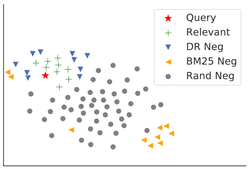
Fig. 24.18 T-SNE representations of query, relevant documents, negative training instances from BM25 (BM25 Neg) or randomly sampled (Rand Neg), and testing negatives (DR Neg) in dense retrieval. Image from [XXL+20].#
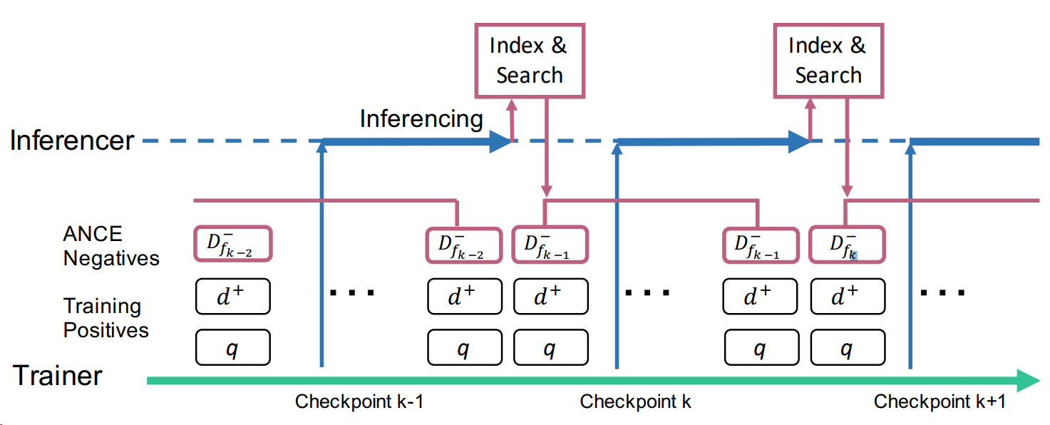
Fig. 24.19 Dynamic hard negative sampling from ANCE asynchronous training framework. Negatives are drawn from index produced using models at the previous checkpoint. Image from [XXL+20].#
RocketQA [QDL+20] follows similar idea in ANCE, but further leverages cross-encoder at the re-ranking stage to generate de-noised hard negatives:
Top-ranked passages from the retriever’s output, excluding the labeled positive passages, are used as hard negatives.
This will bring false negatives since annotators usually only annotate a few top-retrieved passages, therefore the cross-encoder ranker needs to get involve to remove false negatives.
24.5.3.3. Cross-Batch Large-Scale Negatives#
Fundamentally, we want large-scale negatives to better sample the underlying continuous, highdimensional embedding space. In-batch negatives offers an efficient way to construct many negatives during training; however, the number of negatives are limited by GPU memory that determines the batch size. During multiple GPU training [examplified by RocketQA[QDL+20]], in-batch negatives can be generalized to cross-batch negatives to generate large-scale negatives.
Specifically,
We first compute the document embeddings within each single GPU, and then share these documents embeddings among all the GPUs.
Beside in-batch negatives, all documents representations from other GPUs are used as the additional negatives for each query.
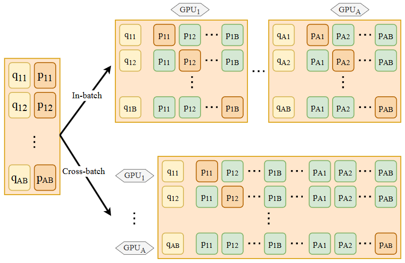
Fig. 24.20 The comparison of in-batch negative and cross-batch negative during multi-gpu training. Image from [QDL+20].#
24.5.3.4. Momentum Negatives#
Even in the single-GPU training setting, we can leverage queue to construct large-scale negatives [MoCo [CFGH20]].
Fundamentally, we want the negatives are coming from the same or similar encoder so that their comparisons in the contrastive learning are consistent.
MoCo leverages an additional momentum network, parameterized by\(\theta_k\), to generate representations that are used as negatives for the main network. The parameters of the key network does not update from graident descent, instead, it is updated from the parameters of the main network network by using a exponential moving average:
where \(m\) is the momentum parameter that takes its value in \([0,1]\). A queue is used to enque representations from the momentum network, which also exits old batch after exceeding queue size. The size of the queue controls the number of negative examples that the main network can see. One example application of Moco is [ICH+21] code
24.5.3.5. Hard Positives#
In the retrieval model query-doc training data, it is usually filled with easy positives, that is query and relevant documents have all query term exact matched. During hybrid retrieval system, as the goal of dense retrieval is to complement sparse retrieval (which relies on exact term matching), it is beneficial to enrich training samples with hard positives, that is query and relevant document does not have all query term exact matched, particularly important query terms. With easy and hard positives, we can design currilumn learning to help model improve its semantic retrieval ability.
24.5.4. Label Denoising#
24.5.4.1. False Negatives#
Hard negative examples produced from static or dynamic negative mining methods are effective to improve the encoder’s performance. However, when selecting hard negatives with a less powerful model (e.g., BM25), we are also running the risk of introduce more false negatives (i.e., negative examples are actually positive) than a random sampling approach. Authors in [QDL+20] proposed to utilize a well-trained, complex model (e.g., a cross-encoder) to determine if an initially retrieved hard-negative is a false negative. Such models are more powerful for capturing semantic similarity among query and documents. Although they are less ideal for deployment and inference purpose due to high computational cost, they are suitable for filtering. From the initially retrieved hard-negative documents, we can filter out documents that are actually relevant to the query. The resulting documents can be used as denoised hard negatives.
24.5.4.2. False Positives#
Because of the noise in the labeling process (e.g., based on click data), it is also possible that a positive labeled document turns out to be irrelevant. To reduce false positive examples, one can develop more robust labeling process and merge labels from multiple sources of signals.
24.5.5. Data Augmentation#
To alleviate the issue of limited labeled training data for bi-encoder, one can leverage the following strategy:
Use existing bi-encoder to retrieve top-\(k\) passages
Use cross-encoder or LLM to denoise generated queries by predicting relevance label, and only pseudo-label positive and negative pair with high-confidence scores.
In the case that we want to adapt a generic retrieval models to a highly specialized domain (e.g., medical, law, scientific), we can consider a LLM-based approach[DZM+22], PROMPTAGATOR, to enhance task-specific retrievers.
As shown in the Fig. 24.21, PROMPTAGATOR consists of three components:
Prompt-based query generation, a task-specific prompt will be combined with a LLM to produce queries for all documents or passages.
Consistency filtering, which cleans the generated data based on round-trip consistency - query should be answered by the passage from which the query was generated. One can also consider other query doc ranking methods in Query-Doc Ranking.
Retriever training, in which a retriever will be trained using the filtered synthetic data.
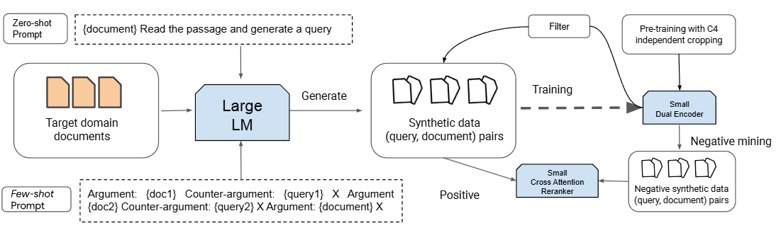
Fig. 24.21 Illustration of PROMPTAGATOR, which generates synthetic data using LLM. Synthetic data, after consistency filtering, is used to train a retriever in labeled data scarcity domain. Image from [DZM+22].#
24.6. Knowledge Distillation#
24.6.1. Introduction#
Knowledge distillation aims to transfer knowledge from a well-trained, high-performing yet cumbersome teacher model to a lightweight student model with significant performance loss. Knowledge distillation has been a widely adopted method to achieve efficient neural network architecture, thus reducing overall inference costs, including memory requirements as well as inference latency. Typically, the teacher model can be an ensemble of separately trained models or a single very large model trained with a very strong regularizer such as dropout. The student model uses the distilled knowledge from the teacher network as additional learning cues. The resulting student model is computationally inexpensive and has accuracy better than directly training it from scratch.
As such, tor retrieval and ranking systems, knowledge distillation is a desirable approach to develop efficient models to meet the high requirement on both accuracy and latency.
For example, one can distill knowledge from a more powerful cross-encoder (e.g., BERT cross-encoder in Section 24.2.3) to a computational efficient bi-encoders. Empirically, this two-step procedure might be more effective than directly training a bi-encoder from scratch.
In this section, we first review the principle of knowledge distillation. Then we go over a couple examples to demonstrate the application of knowledge distillation in developing retrieval and ranking models.
24.6.2. Knowledge Distillation Training Framework#
In the classic knowledge distillation framework [HVD15, TLL+19][Fig. 24.22], the fundamental principle is that the teacher model produces soft label \(q\) for each input feature \(x\). Soft label \(q\) can be viewed as a softened probability vector distributed over class labels of interest. Soft targets contain valuable information on the rich similarity structure over the data. Use MNIST classification as an example, a reasonable soft target will tell that 2 looks more like 3 than 9. These soft targets can be viewed as a strategy to mitigate the over-confidence issue and reduce gradient variance when we train neural networks using one-hot hard labels. Similar mechanism is leveraged in smooth label to improves model generalization.
Allows the smaller Student model to be trained on much smaller data than the original cumbersome model and with a much higher learning rate
Specifically, the logits \(z\) from the techer model are outputted to generate soft labels via
where \(T\) is the temperature parameter controlling softness of the probability vector, and the sum is over the entire label space. When \(T=1\), it is equivalent to standard Softmax function. As \(T\) grows, \(q\) become softer and approaches uniform distribution \(T=\infty\). On the other hand, as \(T\to 0\), the \(q\) approaches a one-hot hard label.
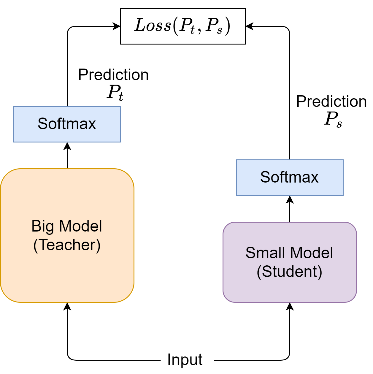
Fig. 24.22 The classic teacher-student knowledge distillation framework.#
The loss function for the student network training is a weighted sum of the hard label based cross entropy loss and soft label based KL divergence. The rationale of KL (Kullback-Leibler) divergence is to use the softened probability vector from the teacher model to guide the learning of the student network. Minimizing the KL divergence constrains the student model’s probabilistic outputs to match soft targets of the teacher model.
The loss function is formally given by
where \(L_{CE}\) is the regular cross entropy loss between predicted probability vector \(p\) and the one-hot label vector
\(L_{KL}\) is the KL divergence loss between the softened predictions at temperature \(T\) from the student and the teacher networks, respectively:
Note that the same high temperature is used to produce distributions from the student model.
Note that \(L_{KL}(p^T, q^T) = L_{CE}(p^T, q^T) + H(q^T, q^T)\), with \(H(q^T, q^T)\) being the entropy of probability vector \(q^T\) and remaining as a constant during the training. As a result, we also often reduce the total loss to
Finally, the multiplier \(T^2\) is used to re-scale the gradient of KL loss and \(\alpha\) is a scalar controlling the weight contribution to each loss.
Besides using softened probability vector and KL divergence loss to guide the student learning process, we can also use MSE loss between the logits from the teacher and the student networks. Specifically, $\(L_{MSE} = ||z^{(T)} - z^{(S)}||^2\)$
where \(z^{(T)}\) and \(z^{(S)}\) are logits from the teacher and the student network, respectively.
Remark 24.3 (connections between MSE loss and KL loss)
In [HVD15], given a single sample input feature \(x\), the gradient of \({L}_{KL}\) with respect to \(z_{k}^{(S)}\) is as follows:
When \(T\) goes to \(\infty\), using the approximation \(\exp \left({z}_{k}/ T\right) \approx 1+{z}_{k} / T\), the gradient is simplified to:
where \(K\) is the number of classes.
Here, by assuming the zero-mean teacher and student logit, i.e., \(\sum_{j} {z}_{j}^{(T)}=0\) and \(\sum_{j} {z}_{j}^{(S)}=0\), and hence \(\frac{\partial {L}_{K L}}{\partial {z}_{k}^{(S)}} \approx \frac{1}{K}\left({z}_{k}^{(S)}-{z}_{k}^{(T)}\right)\). This indicates that minimizing \({L}_{KL}\) is equivalent to minimizing the mean squared error \({L}_{MSE}\), under a sufficiently large temperature \(T\) and the zero-mean logit assumption for both the teacher and the student.
24.6.3. Example Distillation Strategies#
24.6.3.1. Bi-encoder Teacher Distillation#
Authors in [LJZ20, VTGS20] pioneered the strategy of distilling powerful BERT cross-encoder into BERT bi-encoder to retain the benefits of the two model architectures: the accuracy of cross-encoder and the efficiency of bi-encoder.
Knowledge distillation follows the classic soft label framework. Bi-encoder student model training can use pointwise ranking loss, which is equivalent to binary relevance classification problem given a query and a candidate document. More formally, given training examples \((q_i, d_i)\) and their labels \(y_i\in \{0, 1\}\). The BERT cross-encoder as teacher model to produce soft targets for irrelevance label and relevance label.
Although cross-encoder teacher can offer accurate soft labels, it cannot directly extend to the in-batch negatives technique and N-pair loss [Section 24.4.5.1] when training the student model. The reason is that query and document embedding cannot be computed separately from a cross-encoder. Implementing in-batch negatives using cross-encoder requires exhaustive computation on all combinations between a query and possible documents, which amount to \(|B|^2\) (\(|B|\) is the batch size) query-document pairs.
Authors in [LYL21] proposed to leverage bi-encoder variant such as Col-BERT [Section 24.3.2] as a teacher model, which is more feasible to perform exhaustive comparisons between queries and passages since they are passed through the encoder independently [Fig. 24.23].

Fig. 24.23 Compared to cross-encoder teacher, bi-encoder teacher computes query and document embeddings independents, which enables the application of the in-batch negative trick. Image from [LYL21].#
24.6.3.2. Cross-Encoder Embedding Similarity Distillation#
While bi-encoder teacher can offer efficiency in producing on-the-fly teacher scores, it sacrifaces the interaction modeling abiity from cross-encoders. On the other hand, directly using cross-encoder to produce binary classficiation logics as the distillation target does not fully leverage other useful information in the teacher model.
To mitigate this, one can
Having a spealized cross-encoder teacher to produce query and document embeddings
Enforce closeness between student and teacher on query/doc embedding vectors (e.g., via cosine similarity distance)
Enforce closeness between student and teacher on query-doc embedding similarity scores (e.g., via MSE)
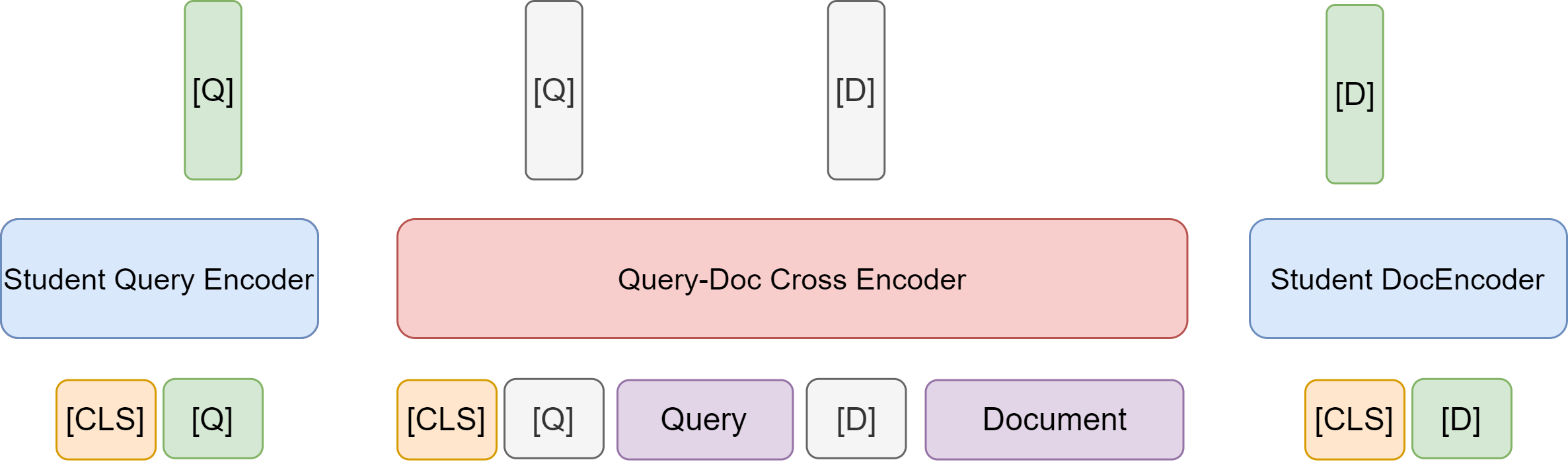
Fig. 24.24 Illustration of leveraging rich information from a cross-encoder teacher for knowledge distillation.#
24.6.3.3. Ensemble Teacher Distillation#
As we have seen in previous sections, large Transformer based models such as BERT cross-encoders or bi-encoders are popular choices of teacher models when we perform knowledge distillation. These fine-tuned BERT models often show high performance variances across different runs. From ensemble learning perspective, using an ensemble of models as a teacher model could potentially not only achieves better distillation results, but also reduces the performance variances.
The critical challenge arising from distilling an ensemble teacher model vs a single teacher model is how to reconcile soft target labels generated by different teacher models.
Authors in [ZQH+21] propose following method to fuse scores and labels. Formally, consider query \(q_{i}\), its \(j\)-th candidate document \(d_{i j}\), and \(K\) teacher models. Let the predicted ranking score by the \(k\)-th teacher be represented as \(\hat{s}_{i j}^{(k)}\).
The simplest aggregated teacher label is to directly use the mean score, namely
The simple average scheme would work poorly when teacher models can have outputs with very different scales. A more robust way to fuse scores is to reciprocal rank, given by
where \(\hat{r}_{i j}^{(k)}\) is the predicted rank of the \(j\)-th candidate text by the \(k\)-th teacher, and \(C\) is the constant as model hyperparameters.
With the fused score, softened probability vector can be obtained by taking Softmax with temperature as the scaling factor.
24.6.3.4. Dynamic Listwise Distillation#
Formally, given a query \(q\) in a query set \(\mathcal{Q}\) and the corresponding list of candidate passages (instance list) \(\mathcal{P}_q=\left\{p_{q, i}\right\}_{1 \leq i \leq m}\) related to query \(q\), we can obtain the relevance scores \(S_{\mathrm{BE}}(q)=\) \(\left\{s_{\mathrm{BE}}(q, p)\right\}_{p \in \mathcal{P}_q}\) and \(S_{\mathrm{CE}}(q)=\left\{s_{\mathrm{ce}}(q, p)\right\}_{p \in \mathcal{P}_q}\) of a query \(q\) and passages in \(\mathcal{P}_q\) from the dual-encoderbased retriever and the cross-encoder-based reranker, respectively. Then, we normalize them in a listwise way to obtain the corresponding relevance distributions over candidate passages:
The main idea is to adaptively reduce the difference between the two distributions from the retriever and the re-ranker so as to mutually improve each other.
To achieve the adaptively mutual improvement, we minimize the KL-divergence between the two relevance distributions \(\left\{\tilde{s}_{\mathrm{BE}}(q, p)\right\}\) and \(\left\{\tilde{s}_{\mathrm{CE}}(q, p)\right\}\) from the two modules:
Additionally, we provide ground-truth guidance for the joint training. Specifically, we can use listwise ranking loss with supervised information:
where \(N\) is the number of training instances, and \(p^{+}\)and \(p^{-}\)denote the positive passage and negative passage in \(\mathcal{P}_q\), respectively. We combine the KL-divergence loss and the supervised crossentropy loss to obtain the final loss function:
24.7. Generalizable Retrievers#
24.7.1. Motivation#
24.7.2. Contriever#
Contriever [ICH+21] explores the limits of contrastive pre-training to learn dense text retrievers. Key tecchniques include positive example generation from unlabeled text, large-scale negative sampling, and pretraining text selection and preparation.
Two positive example generation techniques are considered:
Inverse Cloze Task - Given a sequence of text \(\left(w_1, \ldots, w_n\right)\), ICT samples a span \(\left(w_a, \ldots, w_b\right)\), where \(1 \leq a \leq b \leq n\), uses the tokens of the span as the query and the complement \(\left(w_1, \ldots, w_{a-1}, w_{b+1}, \ldots, w_n\right)\) as the positive example.
Random Cropping - Samples independently two spans from a document to form a positive pair.
To enable the construction of large-scale negative samples, MoCo technique (also see Momentum Negatives) is used to train models with a large number of negative examples. Number of negative examples are ranging from 2,048 to 131,072.
Pretraining dataset consists of Wikipedia and CCNet [WLC+19]. CCNet extracts clean text from Common Crawl wet files and cleans them using a pretrained 5-gram model pretrained on Wikipedia over 18 different languages - by filtering perplexity lower than an given threshold. The model filters out bad quality texts such as code or tables. FastText is used for language identification and deduplication using hash of the content.
Key observations are:
Neural networks trained without supervision using contrastive learning exhibit good retrieval performance, which are competitive with BM25 (albeit not state-of-the-art).
The number of negatives leads to better retrieval performance, especially in the unsupervised setting. However, this effect is not equally strong for all datasets.
These results can be further improved by fine-tuning on the supervised MS MARCO dataset, leading to strong results, in particular for recall@100.
24.7.3. GTR#
Authors from [NQL+21] address the poor ood generalization of typical bi-encoder from perspective of model size and large-scale training. They developped GTR (Generalizable T5-based dense Retrievers), which used T5 encoder as the starting point, and scaling up the size of the bi-encoder model (upto 5B) while keeping the bottleneck embedding size fixed(\(d_m = 768\)).
Besides the model size change, the key recipe in GTR training is large scale data with multi-stage training [Fig. 24.25]:
First stage, contrastive pretraining on input-response pairs and question-answer pairs from online forums and QA websites including Reddit, Stack-Overflow, etc.
Second stage, supervised contrastive finetuning on MS Marco and NQ, with hard negative mining.
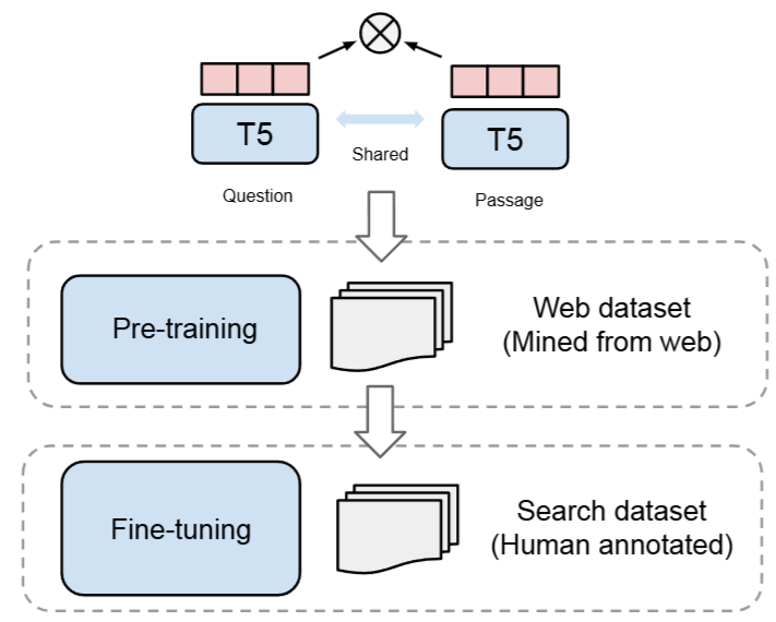
Fig. 24.25 Illutration of GTR retriever two-stage training. Image from [NQL+21].#
Evaluating on the BEIR benchmark (as shown below) shows thatGTR models achieve better out-of-domain NDCG performance when increasing size from Base to XXL [Fig. 24.26].
BM25 |
ColBERT (d=128) |
GTR-Base |
GTR-Large |
GTR-XL |
GTR-XXL |
|
|---|---|---|---|---|---|---|
Model size |
110M |
110M |
335M |
1.34B |
4.8B |
|
Avg |
0.413 |
0.429 |
0.416 |
0.444 |
0.452 |
0.457 |
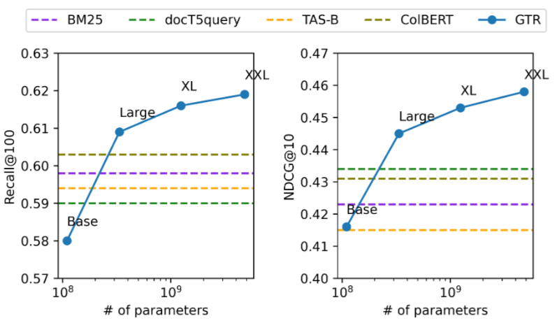
Fig. 24.26 GTR two stage training: contrastive pretraining and supervised finetuning. Image from [NQL+21].#
Further ablation study on the multi-stage training (in the table below) shows that
For fine-tuning only models, scaling up benefits both in-domain and out-of-domain performance.
For pre-training only models, the improvement on in-domain performance is not obvious; meanwhile for out-of-domain tasks, scaling up also improves the generalization.
Combining scaling up and a generic pretraining stage consistently improved fine-tuned-only models.
The gap between GTR (only PT) and GTR also shows the necessity of leveraging a high quality dataset to fine-tune the dual encoders.
Setting |
Model size |
GTR (only FT) |
GTR (only PT) |
GTR |
|---|---|---|---|---|
Indomain Performance (on MS MARCO) |
Base |
0.400 |
0.258 |
0.420 |
Large |
0.415 |
0.262 |
0.430 |
|
XL |
0.418 |
0.259 |
0.439 |
|
XXL |
0.422 |
0.252 |
0.442$ |
|
ood Performance |
Base |
0.387 |
0.295 |
0.416 |
Large |
0.412 |
0.315 |
0.445 |
|
XL |
0.433 |
0.315 |
0.453 |
|
XXL |
0.430 |
0.332 |
0.458 |
24.8. Discussion: Sparse and Dense Retrieval#
Aspects |
BM25 |
Bi-Encoder |
Cross-Encoder |
Late-Interaction BiEncoder (Colbert) |
|---|---|---|---|---|
Speed |
Fast |
Fast |
Slow |
Medium |
Training needed |
N |
Y |
Y |
Y |
OOD Generation |
Strong |
Weak |
Medium |
Medium |
Semantic Understanding |
Weak |
Strong |
Very strong |
Very strong |
Scability |
Y |
Y |
N |
Medium |
Performance |
Consistent medium |
Decent for in-domain |
Strong |
Strong |
In terms of semantic understanding, cross-Encoder sets the upperbound for Late-Interaction Bi-Encoder model.
The importance of Out-of-distribution generation, a robust retriever should have reliable performance on tail topic and tail queries.
When dense model encode a query or document into a fixed length vector, it usually have the following limitations:
Aspects |
Example |
|---|---|
When a query is a short and tail-ish, query embedding is of low quality as the model barely gets exposed to such query during training. |
one word query laresar is a navigation query looking for a Chinese high-tech company. |
When a query is long, specific, and invovles multi-concept with complex relationships or modifiers, the query embedding is insensitive to variations of concept relationships |
The cause of climate change and its impact on marine life in the Altantic sea vs The cause of climate change and its impact on marine life will have high cosine similar embeddings |
What are some good rap songs to dance to? vs What are some of the best rap songs? have high similarity score; but they mean different things. |
|
What are the types of immunity? vs What are the different types of immunity in our body? - the former one is more broad, including immunity in the socieity sense. |
|
Long queries are semantically similar but have many different lexical terms |
What would a Trump presidency mean for current international master’s students on an F1 visa? vs How will a Trump presidency affect the students presently in US or planning to study in US? will have relatively low similarity scores |
Why does China block sanctions at the UN against the Masood Azhar? vs Why does China support Masood Azhar? have low similarity score even if they have the same meaning. |
|
Different query intent due to slight variation on grammar, word order, and word choice |
How do I prevent breast cancer? vs Is breast cancer preventable? have different intent but high similarity score. |
How can I transfer money from Skrill to a PayPal account? vs How can I send money from my PayPal account to my Skrill account to withdraw? have high similarity score, but they mean different directions. Similarly, ‘How do I switch from Apple Music to Spotify?’ vs Should I switch from Spotify to Apple Music? |
|
Queries involving external knowledge that is not in the model |
How do we prepare for UPSC? and How do I prepare for civil service? have low similarity score despite the fact that UPSC and civil service mean the same exam in India |
How competitive is the hiring process at Republic Bank? vs How competitive is the hiring process at S & T Bank? have high similarity score but Republic Bank and S & T bank are different entities. |
|
When a query’s intent shall be interpreted deeply |
My mom wished that I would die has the intent of seeking relationship consultation. |
When a document is long and being compressed into a single dense vector, there will be innevitably information loss.
24.8.1. Index Size and Embedding Dimensionality Impact#
In dense retrieval, query and documents are compressed into low-dimensionality, denoted by \(k\), space. Query and document similarity are computed using length-normalized vectors. Geometrically, each query and documents are residing on the surface of a \(k\)-dimension hyper-space. Intuitively, the larger the index size \(n\) and the smaller \(k\), irrelevant documents more likely to be returned. Authors from [RG20] show that, both theorically and emprically,
The probability of retrieving an irrelevant doc will increase with index size \(n\);
The probability of retrieving an irrelevant doc will increase with dimensionality \(k\).
The emprically findings are summarized in the table below.
Dense Model Setting |
Model |
10k |
100k |
1M |
8.8M |
|---|---|---|---|---|---|
Sparse model |
BM25 |
79.93 |
63.88 |
40.14 |
17.56 |
Trained without hard negatives |
128 dim |
87.50 |
68.63 |
39.76 |
15.71 |
256 dim |
88.82 |
70.79 |
41.74 |
17.08 |
|
768 dim |
88.99 |
71.06 |
42.24 |
17.34 |
|
Trained with hard negatives |
128 dim |
90.32 |
77.92 |
54.45 |
27.34 |
256 dim |
91.10 |
78.90 |
55.51 |
28.16 |
|
768 dim |
91.48 |
79.42 |
56.05 |
28.55 |
24.9. Concept Popularity Bias and Natural Language Query Patterns#
Key findings are [Fig. 24.27]:
DPR performs well on the most common entities but quickly degrades on rarer entities. If the entity is seen in training data, it also tend to perform better than entities it has never seen.
On the other hand, BM25 is less sensitive to entity frequency
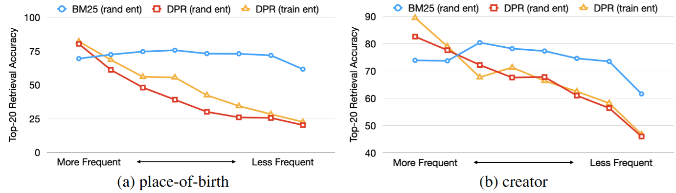
Fig. 24.27 Retrieval accuracy on (a) place-of-birth questions, (b) creator questions, grouped by the entity’s frequency in Wikipedia. rand ent:randomly selected entities from Wikidata; train ent: entities in the NQ training set Image from [SZLC21].#
Question |
Retrieved results from DPR-NQ |
|---|---|
Q: Where was Arve |
Gold: [Title: Arve Furset] Arve Furset Arve Eilif Furset (born 5 December 1964 in |
Top-1: [Title: Gard Agdi] Gard Agdi (“Old Norse” Garðr Agði) appears in the legendary genealogies of “Hversu Noregr byggdist” as one of the three sons of … |
|
Top-2: [Title: Yrsa] kidnapped the queen for a while during which time he made her pregnant. Having returned to her kingdom, the queen bore a child, a girl which she named Yrsa after her dog. Yrsa was sent… |
|
Top-3: [Title: Arvid Noe] Sailor” and the anagram “Arvid Noe” to conceal his identity; his true name, Arne Vidar Røed, became known after his death. Røed began his career as a sailor in 1961, when he… |
FT: fine-tuning on each individual question pattern. w/ similar: fine-tuning on a similar, semantically equivalent question pattern. OnlyP and OnlyQ: fixing the weights of the question encoder and only updating the passage encoder, or vice versa.
bserving the question pattern during training allows DPR to generalize well on unseen entities. On all three relations, DPR can match or even outperform BM25 in terms of retrieval accuracy. Training on the equivalent question pattern achieves comparable performance to the exact pattern, showing dense models do not rely on specific phrasing of the question.
only training the passage encoder (OnlyP) is much more effective than only training the query encoder (OnlyQ)
p-of-birth |
headquarter |
creator |
|
|---|---|---|---|
DPR-NQ |
25.4 |
70.0 |
54.1 |
FT Both |
73.9 |
\(\mathbf{8 4 . 0}\) |
\(\mathbf{8 0 . 0}\) |
FT OnlyP |
\(\mathbf{7 2 . 8}\) |
\(\mathbf{8 4 . 2}\) |
\(\mathbf{7 8 . 0}\) |
FT OnlyQ |
45.4 |
72.8 |
73.4 |
BM25 |
75.2 |
85.0 |
71.7 |
Before fine-tuning, positive passages for place-of-birth questions are clustered together. Discriminating passages in this clustered space is more difficult using an inner product, which explains why only finetuning the question encoder yields minimal gains. After fine-tuning, the passages are distributed more sparsely, making differentiation much easier.
24.10. Approximate Nearest Neighbor Search#
24.10.1. Overview#
Applying dense retrieval in the first-stage of the ad-hoc retrieval system involves performing nearest neighbor search among web-scale documents in the high-dimensional embedding space. Exact nearest neighbor search is inherently expensive due to the curse of dimensionality and the large number of documents. Consider a \(D\)-dimensional Euclidean space \(\mathbb{R}^{D}\), the problem is to find the nearest element \(\mathrm{NN}(x)\), in a finite set \(\mathcal{Y} \subset \mathbb{R}^{D}\) of \(n\) vectors, minimizing the distance to the query vector \(x \in \mathbb{R}^{D}\) is given by:
A brute force exhaustive distance calculation has the complexity of \(\mathcal{O}(n D)\). Several multi-dimensional indexing methods, such as the popular KD-tree [FBF77] or other branch and bound techniques, have been proposed to reduce the search time. However, nowadays the dominating approaches are approximate nearest neighbor search via vector quantization, which is the primary focus of this section.
24.10.2. Vector Quantization#
24.10.2.1. Approximate Representation And Storage#
Quantization is a technique widely used to reduce the cardinality of high dimensional representation space, in particular when the input data is real-valued.
Formally, a quantizer is a function \(q\) mapping a multi-dimensional vector \(x \in \mathbb{R}^{D}\) to a pre-defined centroid \(q(x) = c_i\), where \(c_i \in \mathcal{C} = \{c_1,...,c_{k}\}\). The values \(c_i \in \mathbb{R}^D\) are called centroids, and the set \(\mathcal{C}\) is the codebook of size \(k\).
The set \(\mathcal{V}_{i}\) of vectors mapped to a given index \(i\) is referred to as a (Voronoi) cell, and defined as
The \(k\) cells of a quantizer form a partition of \(\mathbb{R}^{D}\). By definition, all the vectors lying in the same cell \(\mathcal{V}_{i}\) are reconstructed by the same centroid \(c_{i}\). That is, they are all approximated by centroid \(c_i\).
How do we measure the approximation quality of such representation? The quality of a quantizer is usually measured by the mean squared error between the input vector \(x\) and its reproduction value \(q(x):\)
where \(d(x, y)=\|x-y\|\) is the Euclidean distance between \(x\) and \(y\), and where \(p(x)\) is the probability distribution function corresponding the randomly sampled \(x\). Approximate calculation of the integral can be achieved by Monte-Carlo sampling.
In order for the quantizer to be optimal, it has to satisfy two properties known as the Lloyd optimality conditions. First, a vector \(x\) must be quantized to its nearest codebook centroid, in terms of the Euclidean distance:
As a result, the cells are delimited by hyperplanes. The second Lloyd condition is that the reconstruction value must be the expectation of the vectors lying in the Voronoi cell:
The Lloyd quantizer, which corresponds to the \(k\)-means clustering algorithm, finds a near-optimal codebook by iteratively assigning the vectors of a training set to centroids and re-estimating these centroids from the assigned vectors.
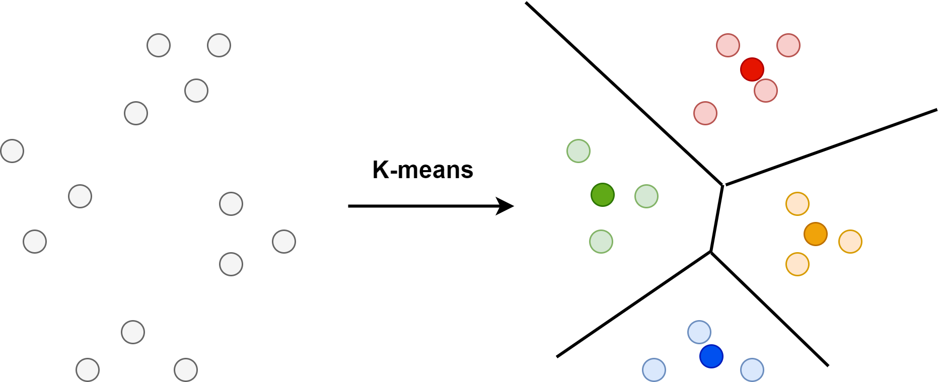
Fig. 24.28 Codecook construction can be achieved using k-means algorithm to compute \(K\) centroids from database vectors.#
The storage for \(N\) vectors now reduce to storage of their index values plus the centroids in the codebook. Each index value requires \(\log_{2} k\) bits. On the other hand, storing the original vectors typically take more than \(\log_2(k)\) bits.
Two important benefits of compressing the dataset are
Memory access times are generally the limiting factor on processing speed; With compression, the processing speed will be drastically accelerated.
Reduce sheer memory capacity for big datasets.
In Fig. 24.29, we illustrate the storage saving by representing a \(D\) dimensional vector by a codebook of 256 centroids. We only need 8-bits (\(2^8 = 256\)) to store a centroid id. Each vector is now replace by a 8-bit integers.
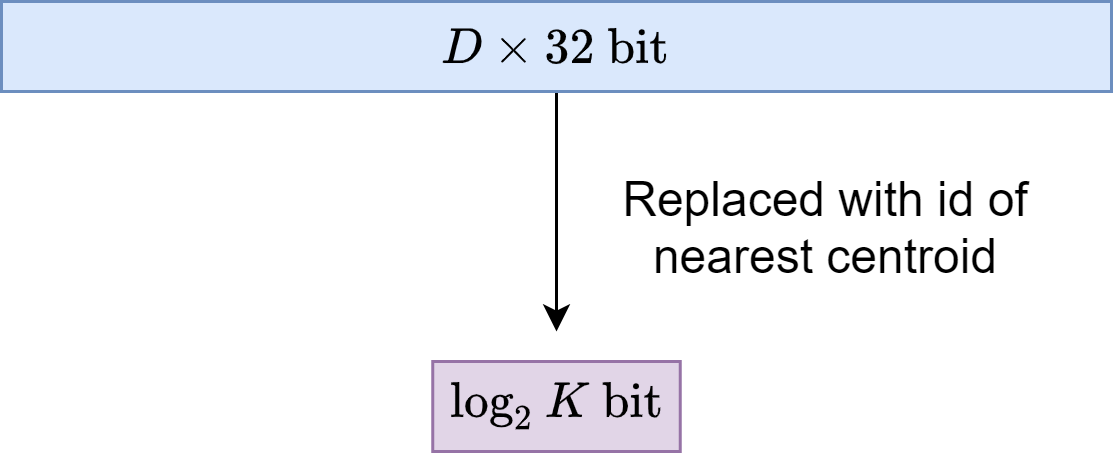
Fig. 24.29 Illustration of memory saving benefits of vector quantization. A \(D\)-dimensional float vector is stored as its nearest centroid integer id, which only occupies \(\log_2 k\) bit.#
24.10.2.2. Approximating Distances Using Quantized Codes#
Given the representation choices for the query vector \(x\) and the database vector \(y\), we define two options in approximating the distance \(d(x, y)\) [Fig. 24.30].
Symmetric distance computation (SDC): both the vectors \(x\) and \(y\) are represented by their respective centroids \(q(x)\) and \(q(y)\). The distance \(d(x, y)\) is approximated by the distance \(\hat{d}(x, y) \triangleq d(q(x), q(y))\).
Asymmetric distance computation (ADC): the database vector \(y\) is represented by \(q(y)\), but the query \(x\) is not encoded. The distance \(d(x, y)\) is approximated by the distance \(\tilde{d}(x, y) \triangleq d(x, q(y))\)
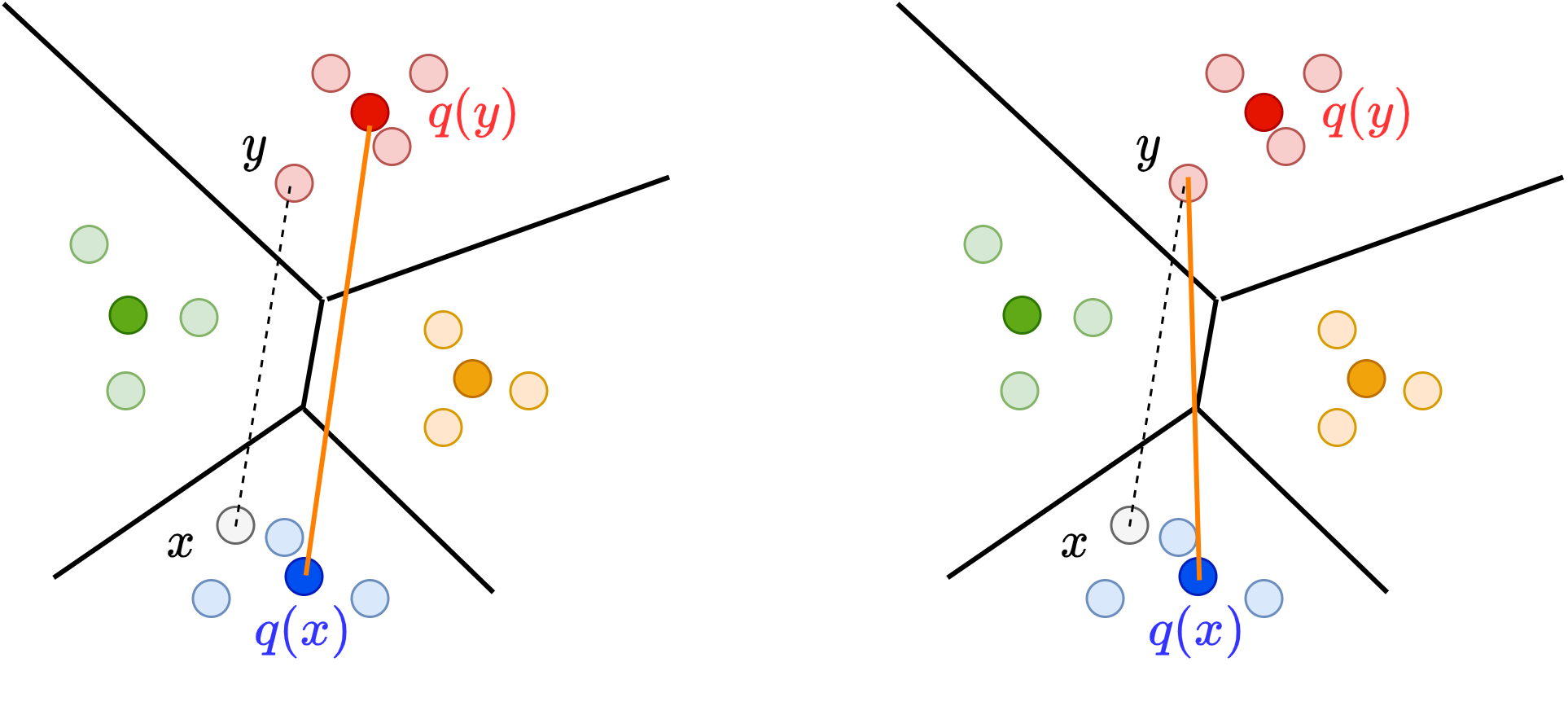
Fig. 24.30 Illustration of the symmetric (left) and asymmetric distance (right) computation. The distance \(d(x, y)\) is estimated with either the distance \(d(q(x), q(y))\) (left) or the distance \(d(x, q(y))\) (right).#
Suppose now we have a query vector \(x\) and we want to find its nearest neighbors among all the \(y\) in the database \(\mathcal{Y}\).
There are benefits in performing symmetric distance computation. To perform symmetric distance computation, we can pre-compute a \(K\times K\) table to cache the Euclidean distance between all centroids. After computing the encoding \(q(x)\), we can get \(d(q(x), q(y))\) by table lookup. On the other hand, to perform asymmetric distance computation between \(x\) and all \(y\in \mathcal{Y}\), we can directly calculate the Euclidean distance between the query vector \(x\) and centroid \(q(y)\) in the codebook.
24.10.3. Product Quantization#
24.10.3.1. From Vector Quantization To Product Quantization#
Let us consider a quantizer producing 64 bits codes, i.e., which can contain \(k=2^{64} \approx 1.8\times 10^{19} \) centroids. It is prohibitive run the k-means algorithm and practically impossible to store the \(D \times k\) floating point values representing the \(k\) centroids.
Product quantization serves as an efficient solution to address these computation and memory consumption issues in vector quantization. The key idea of product quantization is grouping and splitting[ Fig. 24.31]. The input vector \(x\) is split into \(m\) distinct subvectors \(u_{j}, 1 \leq\) \(j \leq m\) of dimension \(D^{*}=D / m\), where \(D\) is a multiple of \(m\). The subvectors are then quantized separately using \(m\) distinct quantizers. A given vector \(x\) is therefore quantized as follows:
where \(q_{j}\) is a quantizer used to quantize the \(j^{\text {th }}\) subvector using the codebook \(\mathcal{C}_{j} = \{c_{j,1},...,c_{j,k^*}\}\). Here we assume that all subquantizers have the same finite number \(k^*\) centroids.
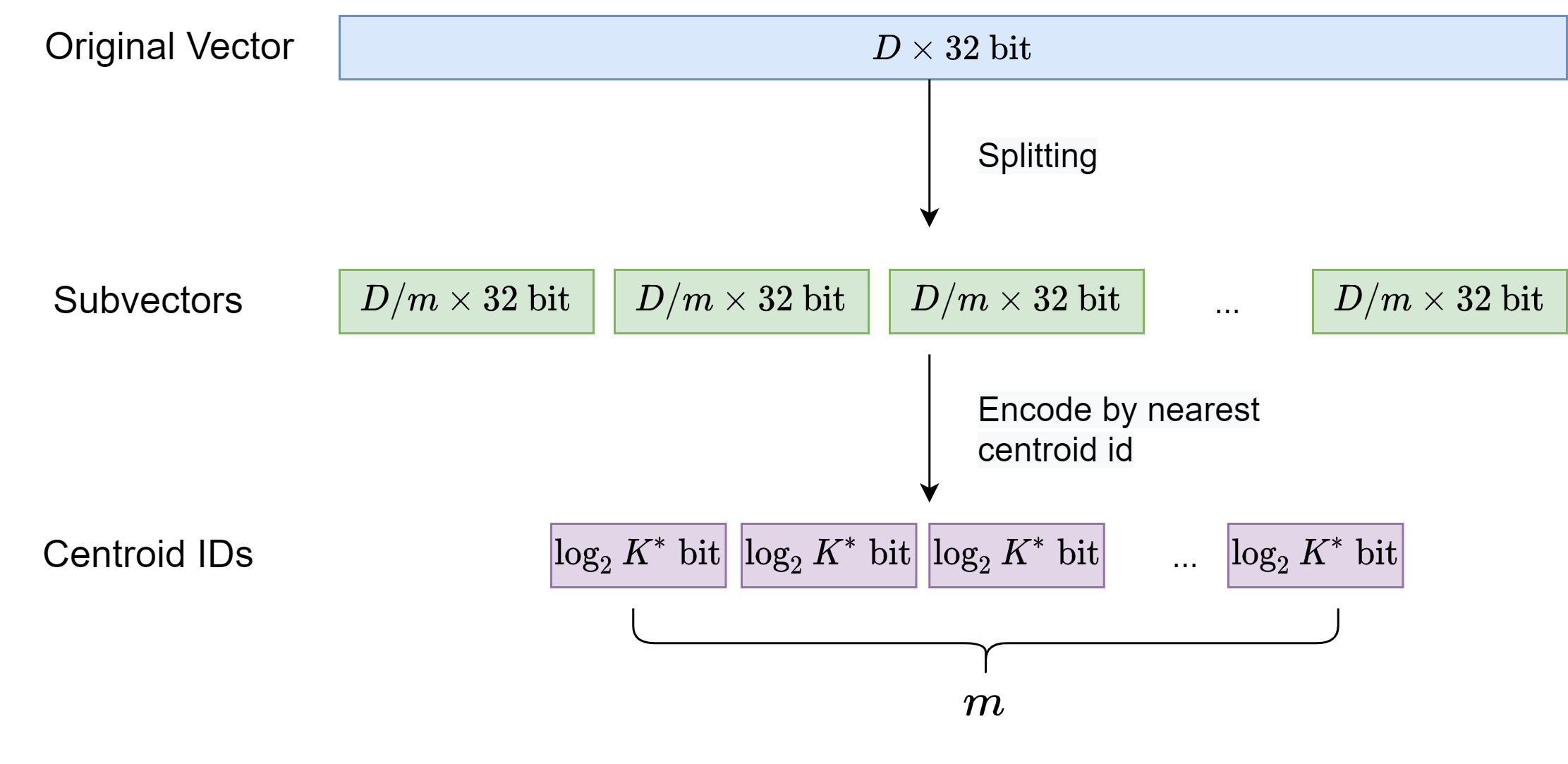
Fig. 24.31 Illustration of memory saving benefits of vector product quantization. A \(D\)-dimensional float vector is first split into \(m\) subvectors, and each subvector is stored as its nearest centroid integer id, which only occupies \(\log_2 K^*\) bit.#
In this case, a reproduction value of the product quantizer is identified by an element of the product index set \(\mathcal{I}=\) \(\mathcal{I}_{1} \times \ldots \times \mathcal{I}_{m}\). The codebook is therefore defined as the Cartesian product
and a centroid of this set is the concatenation of centroids of the \(m\) subquantizers. In that case, the total number of centroids is given by
Note that in the extremal case where \(m=D\), the components of a vector \(x\) are all quantized separately. Then the product quantizer turns out to be a scalar quantizer, where the quantization function associated with each component may be different.
The strength of a product quantizer is to produce a large set of centroids from several small groups of centroids; each group is associated with its own subquantizer.
24.10.3.2. Approximating Distances Using Quantized Codes#
Like vector quantization, we also have different options in approximating distance calculation between query vector \(x\) and database vector \(y\).
Symmetric distance computation (SDC):
where the distance \(d\left(c_{j, i}, c_{j, i^{\prime}}\right)^{2}\) is read from a look-up table associated with the \(j^{\text {th }}\) subquantizer. Each look-up table contains all the squared distances between pairs of centroids \(\left(i, i^{\prime}\right)\) of the subquantizer, or \(\left(k^{*}\right)^{2}\) squared distances \(^{1}\).
Asymmetric distance computation (ADC):
where the squared distances \(d\left(u_{j}(x), c_{j, i}\right)^{2}: j=\) \(1 \ldots m, i=1 \ldots k^{*}\), are computed prior to the search. For nearest neighbors search, we do not compute the square roots in practice: the square root function is monotonically increasing and the squared distances produces the same vector ranking.
24.10.4. Approximate Non-exhaustive Nearest Neighbor Search#
24.10.4.1. Hierarchical Quantization And Inverted File Indexing#
While performing approximate nearest neighbor search with vector quantization or product quantization can already achieve computation acceleration and storage saving in the distance calculation, the search is still exhaustive in which we are computing distance between the query vector and all the vectors in the database. Exhaustive search is not scalable to database containing billions of vectors and scenarios having high query through-puts.
To avoid exhaustive search we can design a hierarchical quantization strategy to reduce the number of candidates that we will run distance calculation and use product quantization to speed up the distance calculation.
The candidate reduction is achieved via a technique called inverted file index (IVF). IVF applies vector quantization via k-means clustering to produce a large number (e.g., 100) of dataset partitions. At the query time, we identify the a number (e.g., 10) of partitions that are the nearest to the query and only compare the query vector to database vector in the these partitions. The residual distance between each vector and its associated partition centroid is approximated by a residual product quantization.
In sparse retrieval, inverted indexing refers to the mapping from a term to a list of documents in the database that contain the term. It resemble the index in the back of a textbook, which maps words or concepts to page numbers
In the context of vector quantization for efficient dense retrieval, we use k-means clustering to partition all vectors in the dataset.
For each partition, an inverted file list refers to the document vectors and its corresponding document ids belonging to this partition.
Given a query, once we determine which partition the query belongs to (using a quantizer), we reduce the search space to the documents in the same partition.
So far, there are two layers of quantization, which are realized through a coarse quantizer and a residual product quantizer. More formally, we denote the centroid \(q_{\mathrm{c}}(y)\) associated with a vector \(y\). Then the product quantizer \(q_{\mathrm{p}}\) is used to encode the residual vector
corresponding to the offset in the Voronoi cell. The energy of the residual vector is small compared to that of the vector itself. The vector is approximated by
Commonly we represent \(y\) by the tuple \(\left(q_{\mathrm{c}}(y), q_{\mathrm{p}}(r(y))\right)\). Like binary representation of a number, the coarse quantizer part represents the most significant bits, while the product quantizer part represents the least significant bits.
Remark 24.4 (shared product quantizer for residuals)
The product quantizer can be learned on a set of residual vectors. Ideally, we can learn a product quantizer for each partition since the residual vectors likely to be dependent on the coarse quantizer. One can further reduce memory cost significantly by using the same product quantizer across all coarse quantizers, although this probably gives inferior results
24.11. Benchmark Datasets#
24.11.1. MS MARCO#
MS MARCO (Microsoft MAchine Reading Comprehension) [NRS+16] is a large scale dataset widely used to train and evaluate models for the document retrieval and ranking tasks as well as tasks like key phrase extraction for question answering. MS MARCO dataset is sampled from Bing search engine user logs, with Bing retrieved passages given queries and human annotated relevance labels. There are more than 530,000 questions in the “train” data partition, and the evaluation is usually performed on around 6,800 questions in the “dev” and “eval” data partition. The ground-truth labels for the “eval” partition are not published. The original data set contains more than \(8.8\) million passages.
There are two tasks: Passage ranking and document ranking; and two subtasks in each case: full ranking and re-ranking.
Each task uses a large human-generated set of training labels. The two tasks have different sets of test queries. Both tasks use similar form of training data with usually one positive training document/passage per training query. In the case of passage ranking, there is a direct human label that says the passage can be used to answer the query, whereas for training the document ranking task we transfer the same passage-level labels to document-level labels. Participants can also use external corpora for large scale language model pretraining, or adapt algorithms built for one task (e.g. passage ranking) to the other task (e.g. document ranking). This allows participants to study a variety of transfer learning strategies.
24.11.1.1. Document Ranking Task#
The first task focuses on document ranking. We have two subtasks related to this: Full ranking and top-100 re-ranking.
In the full ranking (retrieval) subtask, you are expected to rank documents based on their relevance to the query, where documents can be retrieved from the full document collection provided. You can submit up to 100 documents for this task. It models a scenario where you are building an end-to-end retrieval system.
In the re-ranking subtask, we provide you with an initial ranking of 100 documents from a simple IR system, and you are expected to re-rank the documents in terms of their relevance to the question. This is a very common real-world scenario, since many end-to-end systems are implemented as retrieval followed by top-k re-ranking. The re-ranking subtask allows participants to focus on re-ranking only, without needing to implement an end-to-end system. It also makes those re-ranking runs more comparable, because they all start from the same set of 100 candidates.
24.11.1.2. Passage Ranking Task#
Similar to the document ranking task, the passage ranking task also has a full ranking and reranking subtasks.
In context of full ranking (retrieval) subtask, given a question, you are expected to rank passages from the full collection in terms of their likelihood of containing an answer to the question. You can submit up to 1,000 passages for this end-to-end retrieval task.
In context of top-1000 reranking subtask, we provide you with an initial ranking of 1000 passages and you are expected to rerank these passages based on their likelihood of containing an answer to the question. In this subtask, we can compare different reranking methods based on the same initial set of 1000 candidates, with the same rationale as described for the document reranking subtask.
One caveat of the MSMARCO collection is that only contains binary annotations for fewer than two positive examples per query, and no explicit annotations for non-relevant passages. During the reranking task, negative examples are generated from the top candidates of a traditional retrieval system. This approach works reasonably well, but accidentally picking relevant passages as negative examples is possible.
24.11.2. TERC#
24.11.2.1. TREC-deep Learning Track#
Deep Learning Track at the Text REtrieval Conferences (TRECs) deep learning track[^7][CMY+20] is another large scale dataset used to evaluate retrieval and ranking model through two tasks: Document retrieval and passage retrieval.
Both tasks use a large human-generated set of training labels, from the MS-MARCO dataset. The document retrieval task has a corpus of 3.2 million documents with 367 thousand training queries, and there are a test set of 43 queries. The passage retrieval task has a corpus of 8.8 million passages with 503 thousand training queries, and there are a test set of 43 queries.
24.11.2.2. TREC-CAR#
TREC-CAR (Complex Answer Retrieval) [DVRC17] is a dataset where the input query is the concatenation of a Wikipedia article title with the title of one of its sections. The ground-truth documents are the paragraphs within that section. The corpus consists of all English Wikipedia paragraphs except the abstracts. The released dataset has five predefined folds, and we use the first four as a training set (approx. 3M queries), and the remaining as a validation set (approx. 700k queries). The test set has approx. 2,250 queries.
24.11.3. Natural Question (NQ)#
Natural Question (NQ) [KPR+19] introduces a large dataset for open-domain QA. The original dataset contains more than 300,000 questions collected from Google search logs. In [KOuguzM+20], around 62,000 factoid questions are selected, and all the Wikipedia articles are processed as the collection of passages. There are more than 21 million passages in the corpus.
24.11.4. Entity Questions#
[SZLC21]
a set of simple, entityrich questions based on facts from Wikidata (e.g., “Where was Arve Furset born?”)
DPR |
DPR |
BM25 |
|
|---|---|---|---|
Natural Questions |
\(\mathbf{8 0 . 1}\) |
79.4 |
64.4 |
EntityQuestions (this work) |
49.7 |
56.7 |
\(\mathbf{7 2 . 0}\) |
What is the capital of [E]? |
77.3 |
78.9 |
\(\mathbf{9 0 . 6}\) |
Who is [E] married to? |
35.6 |
48.1 |
\(\mathbf{8 9 . 7}\) |
Where is the headquarter of [E]? |
70.0 |
72.0 |
\(\mathbf{8 5 . 0}\) |
Where was [E] born? |
25.4 |
41.8 |
\(\mathbf{7 5 . 3}\) |
Where was [E] educated? |
26.4 |
41.8 |
\(\mathbf{7 3 . 1}\) |
Who was [E] created by? |
54.1 |
57.7 |
\(\mathbf{7 2 . 6}\) |
Who is [E]’s child? |
19.2 |
33.8 |
\(\mathbf{8 5 . 0}\) |
(17 more types of questions) |
\(\cdots\) |
\(\cdots\) |
\(\cdots\) |
24.11.5. BEIR#
BEIR (Benchmarking Information Retrieval) [TRRuckle+21] is a heterogeneous benchmark designed to evaluate zero-shot generalization in retrieval models. It includes 18 datasets across 9 tasks, covering fact-checking, question answering, news retrieval, biomedical IR, and more. The goal is to assess model performance in out-of-distribution (OOD) scenarios, as compared to large, homogeneous datasets like MS MARCO.
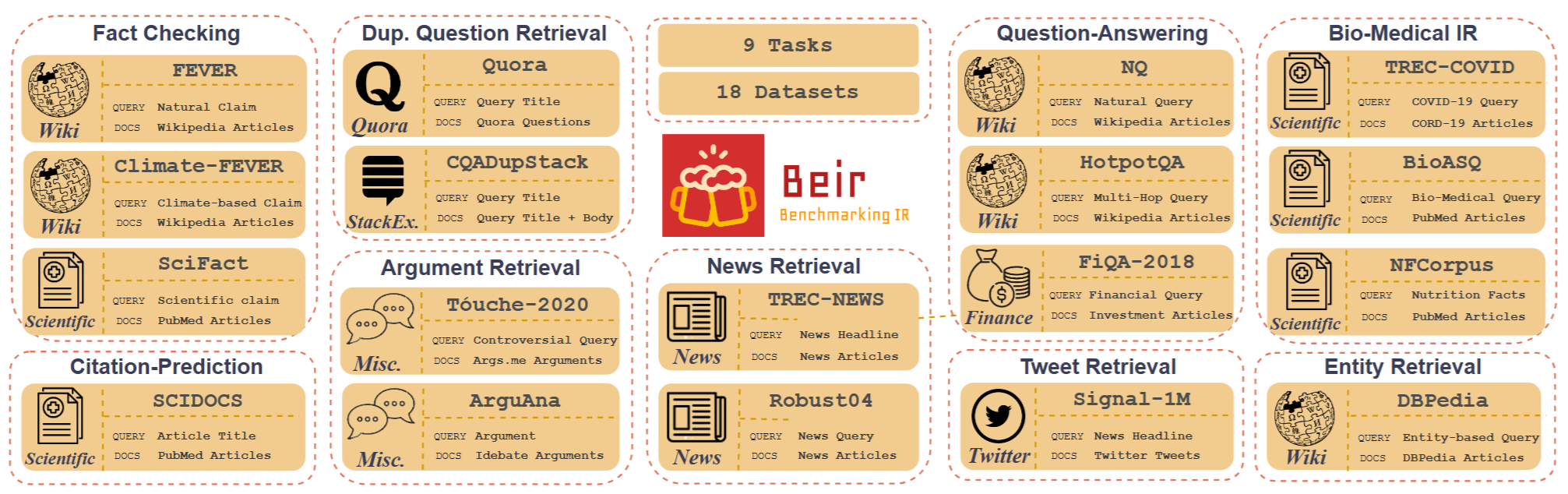
Fig. 24.32 An overview of the diverse tasks and datasets in BEIR benchmark. Image from [TRRuckle+21].#
Dataset |
BEIR-Name |
Type |
Queries |
Corpus |
|---|---|---|---|---|
MSMARCO |
msmarco |
train, dev, test |
6,980 |
8,840,000 |
TREC-COVID |
trec-covid |
test |
50 |
171,000 |
NFCorpus |
nfcorpus |
train, dev, test |
323 |
3,600 |
BioASQ |
bioasq |
train, test |
500 |
14,910,000 |
NQ |
nq |
train, test |
3,452 |
2,680,000 |
HotpotQA |
hotpotqa |
train, dev, test |
7,405 |
5,230,000 |
FIQA-2018 |
fiqa |
train, dev, test |
648 |
57,000 |
Signal-1M(RT) |
signal1m |
test |
97 |
2,860,000 |
TREC-NEWS |
trec-news |
test |
57 |
595,000 |
Robust04 |
robust04 |
test |
249 |
528,000 |
ArguAna |
arguana |
test |
1,406 |
8,670 |
Touche-2020 |
webis-touche2020 |
test |
49 |
382,000 |
CQADupstack |
cqadupstack |
test |
13,145 |
457,000 |
Quora |
quora |
dev, test |
10,000 |
523,000 |
DBPedia |
dbpedia-entity |
dev, test |
400 |
4,630,000 |
SCIDOCS |
scidocs |
test |
1,000 |
25,000 |
FEVER |
fever |
train, dev, test |
6,666 |
5,420,000 |
Climate-FEVER |
climate-fever |
test |
1,535 |
5,420,000 |
SciFact |
scifact |
train, test |
300 |
5,000 |
Key Findings from evaluting BM25 and different dense models:
BM25 remains a strong baseline – Outperforms many neural models across diverse domains in zero-shot settings.
Dense retrieval struggles with generalization – Models like DPR and ANCE often fail on OOD datasets and show a large gap combined to BM25.
Document expansion improves BM25 - Document expansion technique like docT5Query can further improve BM25 across diverse domains.
Trade-off between accuracy and efficiency – Re-ranking models (BM25 + CrossEncoder) or late interaction model like ColBERT perform better than BM25, but are computationally expensive compared to a single sparse and dense models.
Importance of negative sampling and strong teacher distillation - TAS-B, which employed topic-balanced negative sampling and strong teacher distillation, showing the best performance compared to other deep models.
Potential bias towards BM25 - Many benchmarks have relevance labels heavily based on lexical matching, which can disadvantage deep models.
Dataset |
BM25 |
docT5query |
TAS-B |
GenQ |
ColBERT |
BM25+CE |
|---|---|---|---|---|---|---|
MS MARCO (in-domain) |
0.228 |
0.338 |
0.408 |
0.408 |
0.401 |
0.413 |
Quora |
0.789 |
0.802 |
0.835 |
0.830 |
0.854 |
0.825 |
DBPedia |
0.313 |
0.331 |
0.384 |
0.328 |
0.392 |
0.409 |
SciFact |
0.665 |
0.675 |
0.643 |
0.644 |
0.671 |
0.688 |
Avg. Performance vs. BM25 |
+1.6% |
-2.8% |
-3.6% |
+2.5% |
+11% |
24.11.6. LoTTE#
The LoTTE benchmark (Long-Tail Topic-stratified Evaluation for IR) was introduced in [SKSF+21] to complement the out-of-domain tests of BEIR [TRRuckle+21]. LoTTE focuses on natural user queries that pertain to long-tail topics, ones that might not be covered by an entity-centric knowledge base like Wikipedia. LoTTE consists of 12 test sets, each with 500-2000 queries and 100k to 200M passages.
24.11.7. MTEB#
The Massive Text Embedding Benchmark (MTEB) is a large-scale benchmark designed to evaluate the performance of text embedding models across a diverse range of tasks, beyond the text similarity tasks or retrieval tasks. MTEB covers eight embedding tasks spanning 58 datasets in 112 languages, including classification, clustering, retrieval, reranking, pair classification, and summarization.
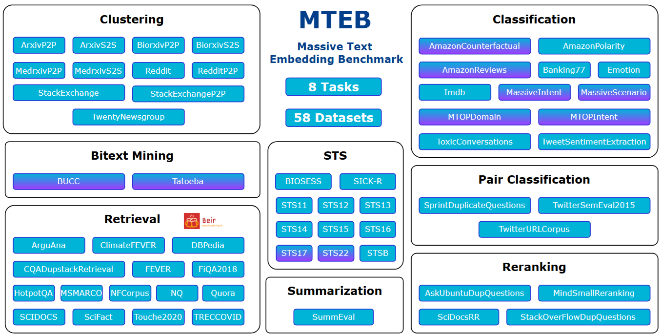
Fig. 24.33 An overview of tasks and datasets in MTEB. Multilingual datasets are marked with a purple shade. Image from [MTMR22].#
No universal best model – No single embedding method consistently outperforms others across all tasks, highlighting the need for task-specific tuning.
Scaling improves performance – Larger models (e.g., ST5-XXL, SGPT-5.8B) generally achieve better results, but at the cost of computational efficiency.
Task specialization matters – ST5 models excel in classification & STS, but perform poorly in retrieval. GTR models dominate retrieval tasks, while struggling in STS. MPNet and MiniLM perform well on reranking and clustering.
Self-supervised models lag behind supervised methods – Unsupervised embeddings like SimCSE-BERT-unsup underperform compared to fine-tuned models.
24.12. Note On Bibliography And Software#
24.12.1. Bibliography#
For excellent reviews in neural information retrieval, see [GFP+20, LNY21, MC+18]
For traditional information retrieval, see [BCC16, CMS10, RZ09, SchutzeMR08]
Qingyao Ai, Xuanhui Wang, Sebastian Bruch, Nadav Golbandi, Michael Bendersky, and Marc Najork. Learning groupwise multivariate scoring functions using deep neural networks. In Proceedings of the 2019 ACM SIGIR international conference on theory of information retrieval, 85–92. 2019.
Christopher JC Burges. From ranknet to lambdarank to lambdamart: an overview. Learning, 11(23-581):81, 2010.
Stefan Buttcher, Charles LA Clarke, and Gordon V Cormack. Information retrieval: Implementing and evaluating search engines. Mit Press, 2016.
Zhe Cao, Tao Qin, Tie-Yan Liu, Ming-Feng Tsai, and Hang Li. Learning to rank: from pairwise approach to listwise approach. In Proceedings of the 24th international conference on Machine learning, 129–136. 2007.
Xinlei Chen, Haoqi Fan, Ross Girshick, and Kaiming He. Improved baselines with momentum contrastive learning. 2020. URL: https://arxiv.org/abs/2003.04297, arXiv:2003.04297.
Nick Craswell, Bhaskar Mitra, Emine Yilmaz, Daniel Campos, and Ellen M Voorhees. Overview of the trec 2019 deep learning track. arXiv preprint arXiv:2003.07820, 2020.
W Bruce Croft, Donald Metzler, and Trevor Strohman. Search engines: Information retrieval in practice. Volume 520. Addison-Wesley Reading, 2010.
Zhuyun Dai, Vincent Y Zhao, Ji Ma, Yi Luan, Jianmo Ni, Jing Lu, Anton Bakalov, Kelvin Guu, Keith B Hall, and Ming-Wei Chang. Promptagator: few-shot dense retrieval from 8 examples. arXiv preprint arXiv:2209.11755, 2022.
Mostafa Dehghani, Hamed Zamani, Aliaksei Severyn, Jaap Kamps, and W Bruce Croft. Neural ranking models with weak supervision. In Proceedings of the 40th International ACM SIGIR Conference on Research and Development in Information Retrieval, 65–74. 2017.
Jacob Devlin, Ming-Wei Chang, Kenton Lee, and Kristina Toutanova. Bert: pre-training of deep bidirectional transformers for language understanding. arXiv preprint arXiv:1810.04805, 2018.
Laura Dietz, Manisha Verma, Filip Radlinski, and Nick Craswell. Trec complex answer retrieval overview. In TREC. 2017.
Jerome H Friedman, Jon Louis Bentley, and Raphael Ari Finkel. An algorithm for finding best matches in logarithmic expected time. ACM Transactions on Mathematical Software (TOMS), 3(3):209–226, 1977.
Jiafeng Guo, Yixing Fan, Liang Pang, Liu Yang, Qingyao Ai, Hamed Zamani, Chen Wu, W Bruce Croft, and Xueqi Cheng. A deep look into neural ranking models for information retrieval. Information Processing & Management, 57(6):102067, 2020.
Ruiqi Guo, Philip Sun, Erik Lindgren, Quan Geng, David Simcha, Felix Chern, and Sanjiv Kumar. Accelerating large-scale inference with anisotropic vector quantization. In International Conference on Machine Learning, 3887–3896. PMLR, 2020.
Dany Haddad and Joydeep Ghosh. Learning more from less: towards strengthening weak supervision for ad-hoc retrieval. In Proceedings of the 42nd International ACM SIGIR Conference on Research and Development in Information Retrieval, 857–860. 2019.
Matthew Henderson, Rami Al-Rfou, Brian Strope, Yun-Hsuan Sung, László Lukács, Ruiqi Guo, Sanjiv Kumar, Balint Miklos, and Ray Kurzweil. Efficient natural language response suggestion for smart reply. arXiv preprint arXiv:1705.00652, 2017.
Geoffrey Hinton, Oriol Vinyals, and Jeff Dean. Distilling the knowledge in a neural network. arXiv preprint arXiv:1503.02531, 2015.
Sebastian Hofstätter, Sheng-Chieh Lin, Jheng-Hong Yang, Jimmy Lin, and Allan Hanbury. Efficiently teaching an effective dense retriever with balanced topic aware sampling. In Proceedings of the 44th International ACM SIGIR Conference on Research and Development in Information Retrieval, 113–122. 2021.
Po-Sen Huang, Xiaodong He, Jianfeng Gao, Li Deng, Alex Acero, and Larry Heck. Learning deep structured semantic models for web search using clickthrough data. In Proceedings of the 22nd ACM international conference on Information & Knowledge Management, 2333–2338. 2013.
Samuel Humeau, Kurt Shuster, Marie-Anne Lachaux, and Jason Weston. Poly-encoders: transformer architectures and pre-training strategies for fast and accurate multi-sentence scoring. arXiv preprint arXiv:1905.01969, 2019.
Gautier Izacard, Mathilde Caron, Lucas Hosseini, Sebastian Riedel, Piotr Bojanowski, Armand Joulin, and Edouard Grave. Unsupervised dense information retrieval with contrastive learning. arXiv preprint arXiv:2112.09118, 2021.
Jeff Johnson, Matthijs Douze, and Hervé Jégou. Billion-scale similarity search with gpus. IEEE Transactions on Big Data, 7(3):535–547, 2019.
Vladimir Karpukhin, Barlas Oğuz, Sewon Min, Patrick Lewis, Ledell Wu, Sergey Edunov, Danqi Chen, and Wen-tau Yih. Dense passage retrieval for open-domain question answering. arXiv preprint arXiv:2004.04906, 2020.
Omar Khattab and Matei Zaharia. Colbert: efficient and effective passage search via contextualized late interaction over bert. In Proceedings of the 43rd International ACM SIGIR conference on research and development in Information Retrieval, 39–48. 2020.
Tom Kwiatkowski, Jennimaria Palomaki, Olivia Redfield, Michael Collins, Ankur Parikh, Chris Alberti, Danielle Epstein, Illia Polosukhin, Jacob Devlin, Kenton Lee, and others. Natural questions: a benchmark for question answering research. Transactions of the Association for Computational Linguistics, 7:453–466, 2019.
Yizhi Li, Zhenghao Liu, Chenyan Xiong, and Zhiyuan Liu. More robust dense retrieval with contrastive dual learning. In Proceedings of the 2021 ACM SIGIR International Conference on Theory of Information Retrieval, 287–296. 2021.
Jimmy Lin, Rodrigo Nogueira, and Andrew Yates. Pretrained transformers for text ranking: bert and beyond. Synthesis Lectures on Human Language Technologies, 14(4):1–325, 2021.
Sheng-Chieh Lin, Jheng-Hong Yang, and Jimmy Lin. In-batch negatives for knowledge distillation with tightly-coupled teachers for dense retrieval. In Proceedings of the 6th Workshop on Representation Learning for NLP (RepL4NLP-2021), 163–173. 2021.
Tianyang Lin, Yuxin Wang, Xiangyang Liu, and Xipeng Qiu. A survey of transformers. arXiv preprint arXiv:2106.04554, 2021.
Wenhao Lu, Jian Jiao, and Ruofei Zhang. Twinbert: distilling knowledge to twin-structured bert models for efficient retrieval. arXiv preprint arXiv:2002.06275, 2020.
Yi Luan, Jacob Eisenstein, Kristina Toutanova, and Michael Collins. Sparse, dense, and attentional representations for text retrieval. Transactions of the Association for Computational Linguistics, 9:329–345, 2021.
Yu A Malkov and Dmitry A Yashunin. Efficient and robust approximate nearest neighbor search using hierarchical navigable small world graphs. IEEE transactions on pattern analysis and machine intelligence, 42(4):824–836, 2018.
Tomas Mikolov, Ilya Sutskever, Kai Chen, Greg S Corrado, and Jeff Dean. Distributed representations of words and phrases and their compositionality. In Advances in neural information processing systems, 3111–3119. 2013.
Bhaskar Mitra, Nick Craswell, and others. An introduction to neural information retrieval. Now Foundations and Trends Boston, MA, 2018.
Niklas Muennighoff, Nouamane Tazi, Loïc Magne, and Nils Reimers. Mteb: massive text embedding benchmark. arXiv preprint arXiv:2210.07316, 2022.
Tri Nguyen, Mir Rosenberg, Xia Song, Jianfeng Gao, Saurabh Tiwary, Rangan Majumder, and Li Deng. Ms marco: a human generated machine reading comprehension dataset. In CoCo@ NIPS. 2016.
Jianmo Ni, Chen Qu, Jing Lu, Zhuyun Dai, Gustavo Hernández Ábrego, Ji Ma, Vincent Y Zhao, Yi Luan, Keith B Hall, Ming-Wei Chang, and others. Large dual encoders are generalizable retrievers. arXiv preprint arXiv:2112.07899, 2021.
Ping Nie, Yuyu Zhang, Xiubo Geng, Arun Ramamurthy, Le Song, and Daxin Jiang. Dc-bert: decoupling question and document for efficient contextual encoding. In Proceedings of the 43rd international ACM SIGIR conference on research and development in information retrieval, 1829–1832. 2020.
Yifan Nie, Alessandro Sordoni, and Jian-Yun Nie. Multi-level abstraction convolutional model with weak supervision for information retrieval. In The 41st International ACM SIGIR Conference on Research & Development in Information Retrieval, 985–988. 2018.
Rodrigo Nogueira and Kyunghyun Cho. Passage re-ranking with bert. arXiv preprint arXiv:1901.04085, 2019.
Rodrigo Nogueira, Wei Yang, Kyunghyun Cho, and Jimmy Lin. Multi-stage document ranking with bert. arXiv preprint arXiv:1910.14424, 2019.
Yingqi Qu, Yuchen Ding, Jing Liu, Kai Liu, Ruiyang Ren, Wayne Xin Zhao, Daxiang Dong, Hua Wu, and Haifeng Wang. Rocketqa: an optimized training approach to dense passage retrieval for open-domain question answering. arXiv preprint arXiv:2010.08191, 2020.
Ori Ram, Gal Shachaf, Omer Levy, Jonathan Berant, and Amir Globerson. Learning to retrieve passages without supervision. arXiv preprint arXiv:2112.07708, 2021.
Nils Reimers and Iryna Gurevych. The curse of dense low-dimensional information retrieval for large index sizes. arXiv preprint arXiv:2012.14210, 2020.
Stephen Robertson and Hugo Zaragoza. The probabilistic relevance framework: BM25 and beyond. Now Publishers Inc, 2009.
Keshav Santhanam, Omar Khattab, Jon Saad-Falcon, Christopher Potts, and Matei Zaharia. Colbertv2: effective and efficient retrieval via lightweight late interaction. arXiv preprint arXiv:2112.01488, 2021.
Hinrich Schütze, Christopher D Manning, and Prabhakar Raghavan. Introduction to information retrieval. Volume 39. Cambridge University Press Cambridge, 2008.
Christopher Sciavolino, Zexuan Zhong, Jinhyuk Lee, and Danqi Chen. Simple entity-centric questions challenge dense retrievers. arXiv preprint arXiv:2109.08535, 2021.
Yelong Shen, Xiaodong He, Jianfeng Gao, Li Deng, and Grégoire Mesnil. A latent semantic model with convolutional-pooling structure for information retrieval. In Proceedings of the 23rd ACM international conference on conference on information and knowledge management, 101–110. 2014.
Kihyuk Sohn. Improved deep metric learning with multi-class n-pair loss objective. Advances in neural information processing systems, 2016.
Hongyin Tang, Xingwu Sun, Beihong Jin, Jingang Wang, Fuzheng Zhang, and Wei Wu. Improving document representations by generating pseudo query embeddings for dense retrieval. arXiv preprint arXiv:2105.03599, 2021.
Raphael Tang, Yao Lu, Linqing Liu, Lili Mou, Olga Vechtomova, and Jimmy Lin. Distilling task-specific knowledge from bert into simple neural networks. arXiv preprint arXiv:1903.12136, 2019.
Nandan Thakur, Nils Reimers, Andreas Rücklé, Abhishek Srivastava, and Iryna Gurevych. Beir: a heterogenous benchmark for zero-shot evaluation of information retrieval models. arXiv preprint arXiv:2104.08663, 2021.
Amir Vakili Tahami, Kamyar Ghajar, and Azadeh Shakery. Distilling knowledge for fast retrieval-based chat-bots. In Proceedings of the 43rd International ACM SIGIR Conference on Research and Development in Information Retrieval, 2081–2084. 2020.
Tongzhou Wang and Phillip Isola. Understanding contrastive representation learning through alignment and uniformity on the hypersphere. In International Conference on Machine Learning, 9929–9939. PMLR, 2020.
Guillaume Wenzek, Marie-Anne Lachaux, Alexis Conneau, Vishrav Chaudhary, Francisco Guzmán, Armand Joulin, and Edouard Grave. Ccnet: extracting high quality monolingual datasets from web crawl data. arXiv preprint arXiv:1911.00359, 2019.
Lee Xiong, Chenyan Xiong, Ye Li, Kwok-Fung Tang, Jialin Liu, Paul Bennett, Junaid Ahmed, and Arnold Overwijk. Approximate nearest neighbor negative contrastive learning for dense text retrieval. arXiv preprint arXiv:2007.00808, 2020.
Jingtao Zhan, Jiaxin Mao, Yiqun Liu, Min Zhang, and Shaoping Ma. Repbert: contextualized text embeddings for first-stage retrieval. arXiv preprint arXiv:2006.15498, 2020.
Honglei Zhuang, Zhen Qin, Shuguang Han, Xuanhui Wang, Michael Bendersky, and Marc Najork. Ensemble distillation for bert-based ranking models. In Proceedings of the 2021 ACM SIGIR International Conference on Theory of Information Retrieval, 131–136. 2021.
24.12.2. Software#
Faiss is a recently developed computational library for efficient similarity search and clustering of dense vectors.