20. Inference Acceleration (WIP)

20.1. The fundamental challenge of LLM inference

20.1.1. Overview

LLM inference is memory-IO bound, not compute bound. In other words, it currently takes more time to load 1MB of data to the GPU’s compute cores than it does for those compute cores to perform LLM computations on 1MB of data.

This is because LLM contains relative usually simple calculations (multiplication, addition, max-pooling, etc) that can be executed by high performing GPU parallel computing units.

This means that LLM inference throughput is largely determined by how large a batch you can fit into high-bandwidth GPU memory.

More specific reasons for LLM inference to be memory-bound is because of the following:

• Model parameters: Modern LLMs often have billions of parameters, requiring significant memory just to store the model weights.

• Attention mechanism: Transformers, which most LLMs are based on, use attention mechanisms that can require large amounts of memory for KV Cache [KV Cache], especially for long sequences.

• Activations: Storing intermediate activations during inference can consume substantial memory.

• Input-output tensors: For autoregressive generation, maintaining the key-value cache for past tokens uses additional memory that grows with sequence length.

While LLM inference is mainly memory-bound, the following factors also contributes to the computation intensity:

Matrix multiplications: The core operations in LLMs are matrix multiplications, which can be computationally intensive. Nonlinear activations: Operations like softmax and layer normalization require additional computation. Beam search: If used, beam search for text generation adds computational overhead.

20.1.2. Memory Requirement Breakdown

Assume every numerical value are stored in \(p\) bytes, we can compute more accurate memory requirements as follows.

Table 20.1 Memory requirement breakdown

Component	Memory Requirement	Note
Model parameter	\(V d+L\left(12 d^2+13 d\right) \times p\)	See Parameter composition in Transformer models
Activations	\(b \times s \times d \times L \times p\)
KV Cache	\(2\times b \times s \times d \times L \times p\)	See KV Cache
Input-output	\(b\times s \times d \times p\)

It is easy to see that domiant memory cost are model paramters and KV Cache.

Example 20.1

20.2. KV Cache

20.2.1. Basics

Key-Value (KV) caching is a crucial optimization technique used in the inference process of Large Language Models (LLMs) to significantly improve performance and reduce computational costs. This technique is particularly important for autoregressive models like GPT, which generate text one token at a time. In transformer-based LLMs, each layer contains self-attention mechanisms that compute attention scores using queries (Q), keys (K), and values (V). During inference, as the model generates each new token, it typically needs to recompute the attention for all previous tokens in the sequence. This process becomes increasingly computationally expensive as the generated sequence grows longer.

KV caching addresses this issue by storing the key and value tensors for each layer of the transformer after they are computed for each token. When generating the next tokens, we need the new token to attend to preceding generated tokens, the model can reuse the cached K and V tensors for these tokens instead of re-computing it. This approach significantly reduces the amount of computation required for each new token, especially for long sequences.

Following Fig. 20.1 illustrate the comparision of the attention computation when generating the second token on the settings of without KV cache and with KV cache.

Particularly, when there is no KV cache and thus previously Key/Value tensors need to be re-computed, and as a result, redundant computation are in every module of the Transformer network:

• Attention layer:

  • As the new token need to attend to all preceding Key/Value tensors and Key/Value tensors are dependent on Query/Key/Value tensors from lower layers, the attention layer simply recompute all steps on the entire sequence, including attention scores and weighted sum of Value (V) vectors.

  • Without KV cache,

• FFN layer & Normalization layer: FFN and Layer Normalization operations in each transformer layer reprocess all previous tokens unnecessarily. With KV cache, these layers only applies to new token’s contextual embedding.

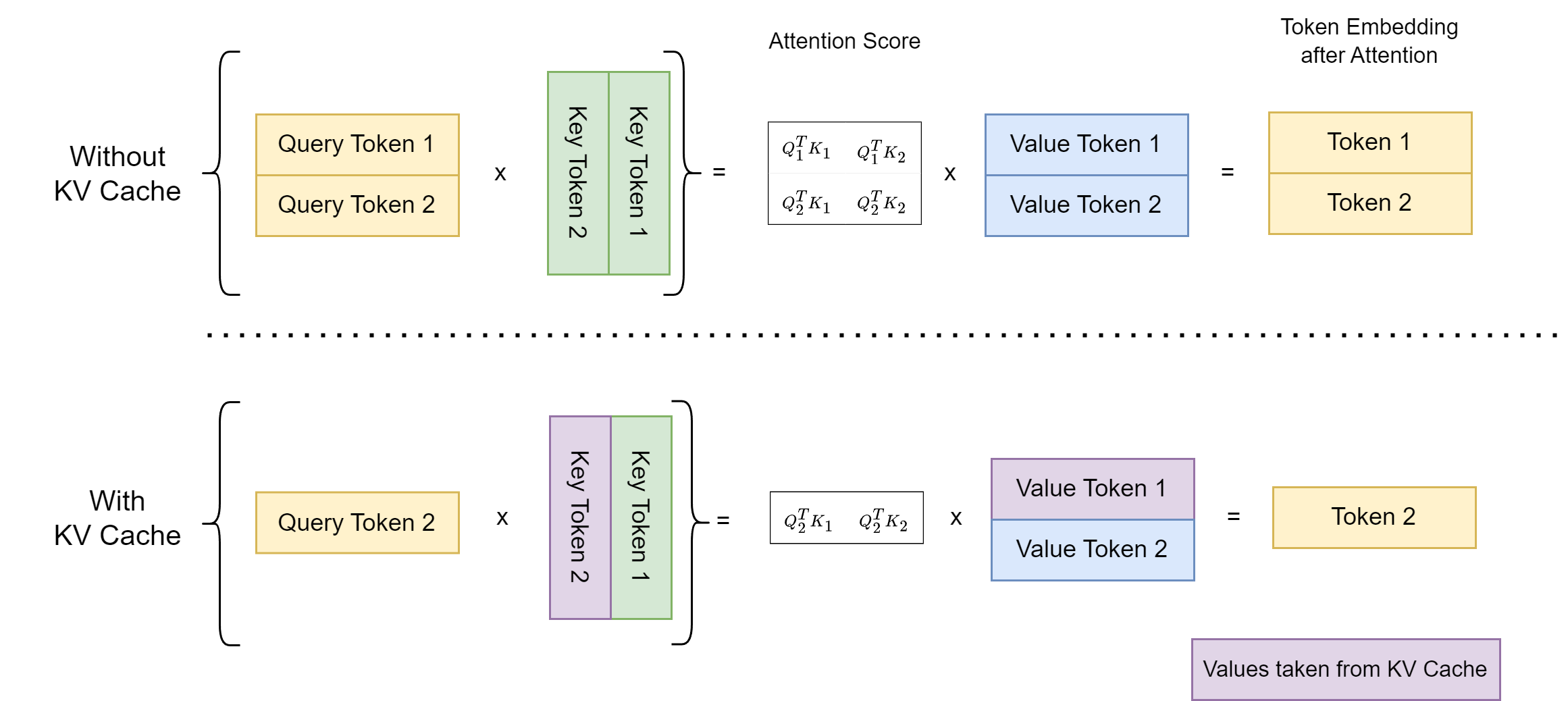
Fig. 20.1 Comparision of the attention computation on the settings of without KV cache and with KV cache.

Benefits

• Faster inference with reduced computational cost: The time complexity for generating each new token becomes constant rather than increasing linearly with sequence length. By reducing redundant computations, KV caching can dramatically speed up the token generation process.

Drawbacks

• Increased memory usage: KV cache is trading inference speed at the cost of memory, which can be substantial for long sequences or large batch sizes.

Remark 20.1 (KV-cache pre-fill for prompts)

While traditional autoregressive generation processes tokens one-by-one, we can prefil KV Cache by leveraging the fact that the prompt is known in advance. Specifically, we can pre-computes and stores the key (K) and value (V) representations for the entire prompt in the cache before generation begins. During token generation, the model can then access these pre-computed values, eliminating the need to recalculate them at each step. This approach reduces computational overhead, especially for tasks involving long prompts or multiple generations from the same context, leading to faster inference times.

20.2.2. Computational cost with KV Cache

In Forward Pass Computation Breadown, we analyze the computational cost during a forward pass without using KV Cache. In this section, we are going to re-analyze the computatioal cost and compare it with the no-KV-Cache setting.

Table 20.2 Computation breakdown

Module	Computation	Matrix Shape Changes	FLOPs (with KV Cache)	FLOPs (without KV Cache baseline)
Attention	\({Q} / {K} / {V}\) Projection	\([{b}, 1, {d}] \times [{~d}, {~d}]\to[{b}, 1, {d}]\)	\(3\times 2 b d^2\)	\(3\times 2 b s d^2\)
	\(Q K^T\)	\([{~b}, 1, {~d}] \times [{~b}, {~d}, (L_{KV} + 1)]\to[{b}, 1, (L_{KV} + 1)]\)	\(2 b d (L_{KV} + 1)\)	\(2 b s^2 d\)
	Score \( \times V\)	\([{~b}, 1, (L_{KV} + 1)] \times [{~b}, (L_{KV} + 1), {~d}]\to[{b}, 1, {d}]\)	\(2 b d (L_{KV} + 1)\)	\(2 b s^2 d\)
	Output (with \(W_o\))	\([{b}, 1, {d}] \times[{~d}, {~d}]\to[{b}, 1, {d}]\)	\(2 b d^2\)	\(2 b s d^2\)
FFN	\(f_1\)	\([{~b}, 1, {~d}] \times[{~d}, 4 {~d}] \to [{b}, 1, 4 {~d}]\)	\(8 b d^2\)	\(8 b s d^2\)
	\(f_2\)	\([{~b}, 1, 4 {~d}] \times[4 {~d}, {~d}]\to[{b}, 1, {d}]\)	\(8 b d^2\)	\(8 b s d^2\)
Embedding		\([{b}, 1, 1] \times[{~V}, {~d}]\to[{b}, 1, {d}]\)	\(2 b d V\)	\(2 b s d V\)
In total			\(\left(24 b d^2+4 b d (L_{KV} + 1) \right) \times L+2 b d V\)	\(\left(24 b s d^2+4 b d s^2\right) \times L+2 b s d V\)

Because \((L_{KV} + 1) = s\), the KV cache reduce the cost to \(1/s\) of the original cost.

20.2.3. Inference Memory Requirement with KV Cache

With KV Cache, the cache memory requirement for inferencing a batch of \(s\)-length sequence is given by

(20.1)\[ M_{KV} = 2\times b \times s \times d \times L \times p \]

where \(b\) is the batch size, \(s\) is the sequence length, \(d\) is the model hidden dim, \(L\) is number of layers, \(p\) is the byte size per model paraemters (e.g., 2 for float16). The multiplier 2 is because of both K and V are cached.

Example 20.2

Consider a model (e.g., Llama7B) with \(d = 4096\), \(s = 2048\), \(b = 64\), and \(L = 32\) = 32. The calculation gives us:

\[M = 2 \times 64 × 2048 × 4096 × 32 × 2 = 68 \text{GB}.\]

As we can see, KV Cache also consumes a significant amount of memory in cases of large batch sizes and long sentences.

68G looks relatively large compared to the model itself, but this is in the case of a large batch. For a single batch, KV Cache would only occupy about 1G of memory, which is just about half the memory of the model parameters.

20.2.4. Combined with GQA

Grouped Query Attention (GQA)[Grouped Query Attention (GQA)] optimizes the computational and memory cost of the regular Multi-head attention (MHA).

For Multi-head attention (MHA), we have \(d = H \times d_{h}\), in which \(H\) is the number of heads, and \(d_h\) is the subspace dimensions of the head. The memory calculation [(20.1)] can also be written by $\( M_{KV} = 2\times b \times s \times H \times d_{H} \times L \times p \)$ Then the GQA memory requirement is given by

(20.2)\[ M_{KV, GQA} = 2\times b \times s \times G \times d_h \times L \times p \]

where \(G\) is the number of Groups. As \(G \ll H\) for large-sized LLM, the savings from GQA can be significant.

20.2.5. Blocked KV Caching via Paged Attention

Traditional LLM inference systems face many inefficiencies in KV-cache memory management. For example, these systems typically pre-allocate contiguous memory chunks based on a request’s maximum length, often leading to inefficient memory utilization:

• The actual request lengths could be much shorter than their maximum potential.

• Even when actual lengths are known in advance, pre-allocation remains inefficient as the entire memory chunk is reserved for the duration of the request, preventing other shorter requests from utilizing unused portions.

There is also a lack of mechnism for memory sharing KV cache for different requests are stored in separate contiguous spaces.

PagedAttention [KLZ+23] is improved memory managment and sharing method. The key idea is that the request’s KV cache is divided into smaller blocks, each of which can contain the attention keys and values of a fixed number of tokens. The benefits are:

• These smaller blocks enable easy use of non-contiguous space, reducing memory fragment waste.

• By using a look-up table to locate the address of each block, the memory sharing and block re-use across different requests can be achieved.

20.3. Quantization Fundamentals

20.3.1. Basic Concepts

Quantization is the process of using a finite number of low-precision values (usually int8) to approximate high-precision (usually float32) numbers with relatively low loss in inference precision.

The objective of quantization is to reduce memory usage and improve inference speed without significantly compromising performance.

In the development of different quantization methods, there are

• QAT (Quantization-Aware-Training), which involves retraining or fine-tuning by approximating the differential rounding operation. While QAT is popular for small neural models, it is rarely used for LLMs.

• PTQ (Post-Training Quantization), which directly quantizes pre-trained LLM models. It requires a small amount of data for determining quantization parameters. This is the mainstream quantization method for LLMs.

Quantization can be applied to different parts of model, including

• weights

• activations

• KV Cache

with different levels of quantization granularities, including:

• per-tensor

• per-token/per-channel

• group-wise

20.3.2. Where quantization and dequant happen? What is the trade off

First a quantized model (together with quantization hypermeters) are loaded into GPU devices (without quantization, the model cannot even be loaded).

During inference calculation, de-quantization is performed when high precision float number calcuation is needed (like Softmax). Note that the majority of inference computation cost is matrix computation, which can usually be conducted via integer level, and half-precision level.

on matrices involved in current step of calculation. After finishing current steps of calcuation, matrices are quantized again to save memory. Since the parameters of the model are not used simultaneously, only part of model parameters are dequantized. Therefore the GPU memory footprint is contained.

Quantization benefits:

• saves the GPU memory footprint,

• calculation speed up with integer level or low precision level matrix computation. Cost:

• with the cost of numerical inaccurcy

• quantization overhead (i.e., convert model weights between)

What Are the Advantages and Disadvantages of Quantized LLMs? Let us look at the pros and cons of quantization.

Pros Smaller Models: by reducing the size of their weights, quantization results in smaller models. This allows them to be deployed in a wider variety of circumstances such as with less powerful hardware; and reduces storage costs.
Increased Scalability: the lower memory footprint produced by quantized models also makes them more scalable. As quantized models have fewer hardware constraints, organizations can feasibly add to their IT infrastructure to accommodate their use. Faster Inference: the lower bit widths used for weights and the resulting lower memory bandwidth requirements allow for more efficient computations. Cons Loss of Accuracy: undoubtedly, the most significant drawback of quantization is a potential loss of accuracy in output. Converting the model’s weights to a lower precision is likely to degrade its performance – and the more “aggressive” the quantization technique, i.e., the lower the bit widths of the converted data type, e.g., 4-bit, 3-bit, etc., the greater the risk of loss of accuracy.

When using a quantized language model (LLM) for inference, there are specific steps where we typically need to de-quantize (or dequantize) the model parameters. Let’s break this down:

1. Storage and Loading: The model parameters remain in their quantized form when stored on disk and when initially loaded into memory.

2. During Forward Pass: a) Weight Matrices: Before matrix multiplications, we usually need to de-quantize the weights. This is because most hardware is optimized for floating-point operations rather than integer operations used in quantized formats.

   b) Attention Mechanisms: For self-attention and cross-attention layers, the key, query, and value matrices typically need to be de-quantized before performing the attention computations.

   c) Layer Normalization: If layer normalization parameters (scale and bias) are quantized, they need to be de-quantized before applying the normalization.

   d) Feed-Forward Networks: The weights of feed-forward layers need to be de-quantized before matrix multiplications.

3. Activation Functions: Generally, activation functions operate on floating-point values, so inputs to these functions (which are outputs from previous layers) need to be in a de-quantized form.

4. Output Layer: The final output layer (e.g., for token prediction) typically works with full-precision values, so any quantized weights here need to be de-quantized.

5. Intermediate Representations: Depending on the specific quantization scheme, some intermediate tensor representations might remain quantized between layers to save memory and computation. These would be de-quantized only when necessary for computations that require higher precision.

It’s important to note that the exact steps where de-quantization occurs can vary depending on:

• The specific quantization scheme used (e.g., INT8, INT4, mixed-precision)

• The hardware being used for inference (some specialized hardware can perform operations directly on quantized values)

• The inference optimization techniques employed (e.g., some frameworks might fuse operations to minimize de-quantization steps)

In practice, many inference engines and frameworks handle these de-quantization steps automatically, optimizing when and where to perform them based on the model architecture and hardware capabilities.

Model quantization is a popular deep learning optimization method in which model data—both network parameters and activations—are converted from a floating-point representation to a lower-precision representation, typically using 8-bit integers. This has several benefits:

When processing 8-bit integer data, NVIDIA GPUs employ the faster and cheaper 8-bit Tensor Cores to compute convolution and matrix-multiplication operations. This yields more compute throughput, which is particularly effective on compute-limited layers. Moving data from memory to computing elements (streaming multiprocessors in NVIDIA GPUs) takes time and energy, and also produces heat. Reducing the precision of activation and parameter data from 32-bit floats to 8-bit integers results in 4x data reduction, which saves power and reduces the produced heat. Some layers are bandwidth-bound (memory-limited). That means that their implementation spends most of its time reading and writing data, and therefore reducing their computation time does not reduce their overall runtime. Bandwidth-bound layers benefit most from reduced bandwidth requirements. A reduced memory footprint means that the model requires less storage space, parameter updates are smaller, cache utilization is higher, and so on.

20.3.3. Standard quantization techniques

To introduce standard quantization techniques, we take 16-bit floating-point model weight \(W_{f16}\) and its quantization into 8-bit integer as example.

The Absmax/Scale quantization technique scales \(W_{f16}\) into the 8-bit representation in the range of \([-127,127]\) via multiplying with

\[s_{W} = \frac{127}{\max_{ij}|W_{f16}|},\]

which is equivalent to scaling the entire tensor to fit into the range of [0, 127]. Specificially, the value with minimal magnitude is mapped to 0 and the value with maximal magnitude is mapped to 127.

That is the 8-bit integer representation is given by

(20.3)\[ W_{i8}=\operatorname{Round}\left(\frac{127 \cdot W_{f16}}{\max_{ij}|W_{f16}|}\right)=\operatorname{Round}\left(s_{W} \mathbf{W}_{f 16}\right) \]

where \(\operatorname{Round}\) indicates rounding to the nearest integer.

The de-quantization of \(W_{i8}\) is given by

\[\operatorname{DeQ}(W_{i8}) = \frac{W_{i8}}{s_{W}}.\]

In practice, there are chances where 8-bit integer value after the quantization is outside of the 8 bit representation. To mitigate this, we will add an additional clipping step,

\[W_{i8} = \]

Affline quantization shifts the input values such that its min value is mapped to -127 and its max value is mapped to 127.

and its into the full range \([-127,127]\) by scaling with the normalized dynamic range \(n d_x\) and then shifting by the zeropoint \(z p_x\). With this affine transformation, any input tensors will use all bits of the data type, thus reducing the quantization error for asymmetric distributions.

For example, for ReLU outputs, in absmax quantization all values in \([-127,0)\) go unused, whereas in zeropoint quantization the full \([-127,127]\) range is used. Zeropoint quantization is given by the following equations:

\[\begin{split} \begin{gathered} n d_{x_{f 16}}=\frac{2 \cdot 127}{\max _{i j}\left(\mathbf{X}_{f 16}^{i j}\right)-\min _{i j}\left(\mathbf{X}_{f 16}^{i j}\right)} \\ z p_{x_{i 16}}=\left\lfloor\mathbf{X}_{f 16} \cdot \min _{i j}\left(\mathbf{X}_{f 16}^{i j}\right)\right\rceil \\ \mathbf{X}_{i 8}=\left\lfloor n d_{x_{f 16}} \mathbf{X}_{f 16}\right\rceil \end{gathered} \end{split}\]

The Round-to-Nearest (RTN) quantization is a basic method used in the process of quantizing neural networks.

For a given numerical value \(r\), RTN applies the following quantization formula

\[q = \operatorname{Clip}(\operatorname{Round}(\frac{r}{s}) + z, q_{min}, q_max)\]

where \(s\) is scaling parameter, \(z\) is the shifting parameter, and \(q_{min}, q_{max}\) are the clipping range.

20.3.4. Quantized matrix multiplication

The modern GPU hardware can significantly speed up the matrix multiplication in the integer representation. As matrix multiplication involves accumulation operations, the typical convension for accumulation data types are

Low-Precision Data Type	Accumulation Data Type
float16	float16
bfloat16	float32
int16	int32
int8	int32

The matrix multiplication between \(X_{f16}\) and \(W_{f16}\) can be approximated by

\[\begin{split} \begin{aligned} X_{f16}W_{f16} &\approx \operatorname{DeQ}(X_{i8}) \operatorname{DeQ}(W_{i8}) \\ &=\frac{X_{i8}}{s_{X}} \frac{W_{i8}}{s_{W}} \\ &=\frac{1}{s_{X}\cdot s_W} X_{i8}W_{i8} \end{aligned} \end{split}\]

where the summation or accumation operation in matrix multiplication of \(X_{i8}W_{i8}\) will be conducted in int-32 data type.

20.3.5. Quantization granularities

These different granularities offer trade-offs between quantization accuracy and computational efficiency. Per-tensor is the fastest but least accurate, per-channel/per-token is the most accurate but computationally expensive, and group-wise provides a balance between the two extremes

Per-tensor quantization applies the same scaling factor and zero point to an entire tensor (usually a weight matrix or activation tensor). Each weight tensor and activation tensor in the model will have its own set of quantization parameters. Note that the biggest challenges for per-tensor quantization is that a single outlier can reduce the quantization precision of all other values.

Example 20.3 (Per-tensor quantization)

Let’s consider a weight matrix \(W\), the quantize \(W\) into int8, we have the following steps:

1. Find the minimum and maximum values in the entire tensor: min_val = -0.5, max_val = 0.8

2. Calculate the scale and zero point: scale = (max_val - min_val) / (2^8 - 1) = (0.8 - (-0.5)) / 255 ≈ 0.00510 zero_point = round(-min_val / scale) = round(0.5 / 0.00510) ≈ 98

3. Quantize the entire tensor using these parameters: W_quant = round(W / scale) + zero_point

In this case, all elements use the same scale (0.00510) and zero_point (98) for quantization and dequantization.

Per-channel (from model weights perspective) quantization applies different scaling factors and zero points to each channel in the tensor. Explanation: This method computes separate quantization parameters for each channel (in the case of weights) or each token (in the case of activations). This allows for more fine-grained quantization, potentially preserving more information.

Example 20.4 (Per-channel quantization)

Let’s consider the same weight matrix \(W\) of shape (1024, 768), but now we’ll quantize each output channel separately.

To quantize this to int8 per-channel, for each of the 768 columns (channels):

1. Find the minimum and maximum values in that column

2. Calculate the scale and zero point for that column

3. Quantize the column using its specific parameters

Each column in W_quant uses its own scale and zero_point for quantization and dequantization.

Per-token (from activations perspective) quantization applies different scaling factors and zero points to each token in the tensor.

For a given activation tensor \(A\) of shape \((B, S, H)\), where:

• \(B\) is the batch size

• \(S\) is the sequence length

• \(H\) is the hidden dimension

There will be \(S\) sets of quantization parameters; each set of parameters is computed from the \(H\) hidden dimensionality values.

20.3.6. Groupwise quantization

20.3.7. Quantization-performance trade-off in language models

Early research [[BNB21]] during the BERT era revealed significant challenges in quantizing large language models. [BNB21] demonstrated that applying round-to-nearest (RTN) quantization to both weights and activations of BERT models, reducing them to 8-bit precision, resulted in substantial performance deterioration on language understanding benchmarks.

Further ablation shows that quantization on activation is major cause of the performance drop and quantization on the model weights have minimal impact. The reason is that activation values from FFN’s input and output can have strong outliers, which can directly cause notable error in the quantization process.

As summary in the following table [[BNB21]], a strategy of quantizing only the model weights to 8-bit precision while maintaining 32-bit precision for activations (referred to as ‘W8A32’) achieved performance comparable to full-precision models. This finding highlights the importance of selective quantization strategies that preserve critical information in activations while still benefiting from the efficiency gains of weight quantization.

Configuration	CoLA	SST-2	MRPC	STS-B	QQP	MNLI	QNLI	RTE	GLUE
FP32	57.27	93.12	88.36	89.09	89.72	84.91	91.58	70.40	83.06
W8A8	54.74	92.55	88.53	81.02	83.81	50.31	52.32	64.98	71.03
W32A8	56.70	92.43	86.98	82.87	84.70	52.80	52.44	53.07	70.25
W8A32	58.63	92.55	88.74	89.05	89.72	84.58	91.43	71.12	83.23

As the model size continues to grow to billions of parameters, outlier features of high magnitude start to emerge in all transformer layers, causing failure of simple low-bit quantization. Dettmers et al. (2022) observed such a phenomenon for OPT models larger than 6.7B parameters. Larger models have more layers with extreme outliers and these outlier features have a significant impact on the model performance. The scale of activation outliers in a few dimensions can be \(\sim 100 \times\) larger than most of the other values.

As language models grow to encompass billions of parameters, a significant challenge emerges: the appearance of high-magnitude outlier features across all transformer layers. This phenomenon compromises the effectiveness of simple low-bit quantization techniques. [DLBZ22] identified this issue in OPT models exceeding 6.7 billion parameters.

The problem intensifies with model size; larger models exhibit more layers with extreme outliers. These outlier features disproportionately influence model performance. In some dimensions, the scale of activation outliers can be approximately 100 times larger than the majority of other values.

This disparity poses a significant challenge for quantization, as traditional methods struggle to accurately represent both the outliers and the more typical values within the same low-bit format. Consequently, addressing these outliers has become a critical focus in the development of quantization techniques for large language models.

20.4. Advanced quantization techniques

20.4.1. LLM.int8()

[DLBZ22]

Motivation

Basic quantization methods often resulted in significant performance degradation, especially for larger models.

maintain high performance while significantly reducing the memory footprint and computational requirements of large language models. This makes it possible to run these models on more modest hardware or to scale them more efficiently in production environments.

The key idea is:

• Group-wise quantization: Instead of quantizing the entire model uniformly, the method divides weight matrices into groups and quantizes each group separately. This allows for more fine-grained representation of the weights.

• Outlier handling: The method identifies and separates outlier values before quantization. These outliers are stored in 16-bit precision, while the rest of the weights are quantized into 8-bit int.

Method details:

For a given input matrix \(\mathbf{X}_{f 16} \in \mathbb{R}^{s \times h}\),

• First identify the subset of hidden dimensions that have at least one outliers based on certain magnitude criterion. We denote these dimensions by \(O=\{i \mid i \in \mathbb{Z}, 0 \leq i \leq h\}\).

• For columns of \(X\) and rows in \(W\) that reside in \(O\), we preserve its 16-bit precision; for the remaining columns and rows, we quantize into 8-bit precision.

• The final resulting matrix can be represented by the adding inner products together, that is

\[ \mathbf{C}_{f 16} \approx \sum_{h \in O} \mathbf{X}_{f 16}^h \mathbf{W}_{f 16}^h+\mathbf{S}_{f 16} \cdot \sum_{h \notin O} \mathbf{X}_{i 8}^h \mathbf{W}_{i 8}^h \]

where \(\mathbf{S}_{f 16}\) is the denormalization term for the Int8 inputs and weight matrices \(\mathbf{X}_{i 8}\) and \(\mathbf{W}_{i 8}\).

It is found that 99.9% values can be represented by 8-bit int.

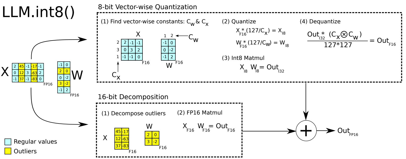
Fig. 20.2 Figure 2: Schematic of LLM.int8(). Given 16-bit floating-point inputs \(\mathbf{X}_{f 16}\) and weights \(\mathbf{W}_{f 16}\), the features and weights are decomposed into sub-matrices of large magnitude features and other values. The outlier feature matrices are multiplied in 16 -bit. All other values are multiplied in 8 -bit. We perform 8 -bit vector-wise multiplication by scaling by row and column-wise absolute maximum of \(\mathbf{C}_x\) and \(\mathbf{C}_w\) and then quantizing the outputs to Int8. The Int32 matrix multiplication outputs \(\mathrm{Out}_{i 32}\) are dequantization by the outer product of the normalization constants \(\mathbf{C}_x \otimes \mathbf{C}_w\). Finally, both outlier and regular outputs are accumulated in 16-bit floating point outputs. Image from [DLBZ22].

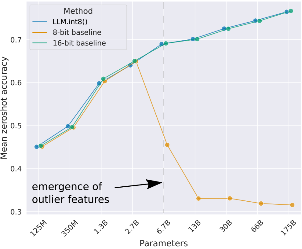
Fig. 20.3 OPT model mean zeroshot benchmark accuracy at different quantization settings, including 16-bit baseline, regular 8-bit quantization method, and the LLM.int8() quantization method. Systematic outliers emerge at a scale of 6.7B parameters, causing regular quantatization methods to have severe performance degradation. Image from [DLBZ22].

20.4.2. Smooth Quant

20.4.3. AWQ

20.4.4. GPTQ

20.4.4.1. The Error Minimization Framework

[LDS89]

If we want to remove some parameters from a model (i.e., pruning), intuitively, we want to remove parameters that have little impact on the objective function \(E\). So we can perform a Taylor expansion on the objective function \(E\):

(20.4)\[ \Delta E=\sum_i g_i \Delta w_i+\frac{1}{2} \sum_i h_{ii} \Delta w_i^2+\frac{1}{2} \sum_{i \neq j} h_{ij} \Delta w_i \Delta w_j+O\left(\Delta w^3\right) \]

where \(g_i=\frac{\partial E}{\partial w_i}\) is the first-order partial derivative of the parameter, and \(h_{ij}=\frac{\partial^2 E}{\partial w_i \partial w_j}\) is an element of the Hessian matrix.

We can make the following some assumptions to simplify the above equation and facilate our subsequent analysis

• The contribution from higher-order terms \(O\left(\Delta w^3\right)\) can be ignored

• The model training has converged sufficiently, so all first-order partial derivatives of parameters are 0: \(g_i=0, \forall i\)

This reduces the original \(\Delta E\) expression to

(20.5)\[ \Delta E=\frac{1}{2} \sum_i h_{ii} \Delta w_i^2+\frac{1}{2} \sum_{i \neq j} h_{ij} \Delta w_i \Delta w_j \]

20.4.4.2. Speical Case: Diagonal Hessian Assumption

One special case is when the Hessian matrix is a diagnoal, that is, the impact of each parameter on the objective function is independent. As a result \(h_{ij}\Delta w_i \Delta w_j = 0\), the Eq. (20.5) can be simplified to:

\[ \Delta E=\frac{1}{2} \sum_i h_{ii} \Delta w_i^2. \]

From this equation, the impact of deleting a parameter \(w_i\) on the objective function is \(\frac{1}{2} h_{ii} w_i^2\). So we only need to calculate the Hessian matrix \(h_{ii}\) to know the impact of each parameter on the objective. Then we can rank the parameters according to their impact from small to large, which determines the order of parameter pruning.

20.4.4.3. General Case

OBS [HSW93]

To analyze the general case of Eq. (20.5), we first write it in vector/matrix form: $\( \Delta E=\frac{1}{2} \Delta \mathbf{w}^{\mathbf{T}} \mathbf{H} \Delta \mathbf{w} \)$ (chapter_inference_eq_inference_acceleration_GPTQ_error_minimization_objective_matrix_form)

When deleting a weight \(w_q\), the \(q\)-th dimension of \(\Delta \mathbf{w}\) is fixed at \(-w_q\), but the values in other dimensions can vary and can be used to reduce the deviation from the objective caused by deleting this weight.

The \(q\)-th dimension of \(\boldsymbol{\Delta} \mathbf{w}\) being fixed at \(-w_q\) is a constraint condition, which we can express as an equation:

\[ \mathbf{e}_{\mathbf{q}}^{\mathbf{T}} \cdot \boldsymbol{\Delta} \mathbf{w}+w_q=0 \]

where \(\mathbf{e}_{\mathbf{q}}\) is a one-hot vector with 1 at the \(q\)-th position and 0 elsewhere.

We want to find the most suitable weight \(w_q\) to delete, which minimizes the impact on the objective. This can be expressed as an optimization problem:

\[ \min_{\Delta \mathbf{w}, q} \frac{1}{2} \boldsymbol{\Delta}_{\mathbf{w}}^{\mathbf{T}} \mathbf{H} \boldsymbol{\Delta} \mathbf{w} \quad \text{s.t.} \quad \mathbf{e}_{\mathbf{q}}^{\mathbf{T}} \cdot \boldsymbol{\Delta} \mathbf{w}+w_q=0 \]

Solving this using the Lagrange multiplier method:

\[ \Delta \mathbf{w}=-\frac{w_q}{[\mathbf{H}^{-1}]_{qq}} \mathbf{H}^{-1} \cdot \mathbf{e}_{\mathbf{q}} \]

And the error function with optimal \(\Delta \mathbf{w}\) is given by

\[\Delta E =\frac{1}{2} \frac{w_q^2}{[\mathbf{H}^{-1}]_{qq}}\]

Detailed Derivation

Step 1: Form the Lagrangian Let’s introduce a Lagrange multiplier \(\lambda\) and form the Lagrangian function:

\[ L(\boldsymbol{\Delta}\mathbf{w}, \lambda) = \frac{1}{2} \boldsymbol{\Delta}\mathbf{w}^{T} \mathbf{H} \boldsymbol{\Delta}\mathbf{w} + \lambda(\mathbf{e}_{q}^{T} \cdot \boldsymbol{\Delta}\mathbf{w}+w_q) \]

Step 2: Find the partial derivatives and set them to zero

With respect to \(\boldsymbol{\Delta}\mathbf{w}\) and \(\lambda\):

\[\begin{split} \begin{align} \frac{\partial L}{\partial \boldsymbol{\Delta}\mathbf{w}} &= \mathbf{H}\boldsymbol{\Delta}\mathbf{w} + \lambda\mathbf{e}_{\mathbf{q}} = 0 \\ \frac{\partial L}{\partial \lambda} &= \mathbf{e}_{\mathbf{q}}^{\mathbf{T}} \cdot \boldsymbol{\Delta}\mathbf{w}+w_q = 0 \end{align} \end{split}\]

Step 3: From the first equation we get $\( \boldsymbol{\Delta}\mathbf{w} = -\lambda \mathbf{H}^{-1}\mathbf{e}_q \)$

Plus into the second

\[ -\lambda \mathbf{e}_q^T\mathbf{H}^{-1}\mathbf{e}_q + w_q = 0 \implies \lambda = \frac{w_q}{[\mathbf{H}]^{-1}_{qq}} \]

where \([\mathbf{H}]^{-1}_{qq}\) is the \(q\)-th diagonal element of \(\mathbf{H}^{-1}\)

Now the first equation becomes

\[ \mathbf{H}\boldsymbol{\Delta}\mathbf{w} + \frac{w_q}{[\mathbf{H}^{-1}]{qq}}\mathbf{e}_q = 0 \]

from which we can solve \(\boldsymbol{\Delta}\mathbf{w}\) to get

\[ \boldsymbol{\Delta}\mathbf{w} = -\frac{w_q}{[\mathbf{H}^{-1}]{qq}}\mathbf{H}^{-1}\mathbf{e}_q \]

The implication is that the impact of pruning parameter \(w_q\) is \(\frac{1}{2} \frac{w_q^2}{[\mathbf{H}^{-1}]_{qq}}\). So our pruning algorithm can be conducted by iteratively pruning parameters that has minimal impact and adjusting remaining parameters to offset the impact, as we summarize below.

Algorithm 20.1 (OBS Neural Network Pruning Algorithm)

Inputs A trained neural network; Stop Criterion

Output A pruned neural network

1. Compute \(\mathbf{H}^{-1}\).

2. Find the \(q\) that gives the smallest saliency \(L_q=u_q^2 /\left(2\left[\mathbf{H}^{-1}\right] q q\right)\). If this candidate error increase is much smaller than \(E\), then the \(q\) th weiglit should be deleted, and we proceed to step 4: otherwise go to step 5. (Other stopping criteria can be used too.)

3. Use the \(q\) from step 3 to update all weights (Eq. 5). Go to step 2.

4. No more weights can be deleted without large increase in E. (At this point it may be desirable to retrain the network.)

20.4.4.4. Speed-Up Hessian Computation

20.5. Prompt Compression

[JWL+23]

20.6. FP8

20.7. Bibliography

Additional References and software

https://lilianweng.github.io/posts/2023-01-10-inference-optimization/

Quantization: https://leimao.github.io/article/Neural-Networks-Quantization/

[BNB21] (1,2,3)

Yelysei Bondarenko, Markus Nagel, and Tijmen Blankevoort. Understanding and overcoming the challenges of efficient transformer quantization. 2021. URL: https://arxiv.org/abs/2109.12948, arXiv:2109.12948.

[DLBZ22] (1,2,3,4)

Tim Dettmers, Mike Lewis, Younes Belkada, and Luke Zettlemoyer. Llm.int8(): 8-bit matrix multiplication for transformers at scale. 2022. URL: https://arxiv.org/abs/2208.07339, arXiv:2208.07339.

[HSW93]

Babak Hassibi, David G Stork, and Gregory J Wolff. Optimal brain surgeon and general network pruning. In IEEE international conference on neural networks, 293–299. IEEE, 1993.

[JWL+23]

Huiqiang Jiang, Qianhui Wu, Chin-Yew Lin, Yuqing Yang, and Lili Qiu. Llmlingua: compressing prompts for accelerated inference of large language models. arXiv preprint arXiv:2310.05736, 2023.

[KLZ+23]

Woosuk Kwon, Zhuohan Li, Siyuan Zhuang, Ying Sheng, Lianmin Zheng, Cody Hao Yu, Joseph Gonzalez, Hao Zhang, and Ion Stoica. Efficient memory management for large language model serving with pagedattention. In Proceedings of the 29th Symposium on Operating Systems Principles, 611–626. 2023.

[LDS89]

Yann LeCun, John Denker, and Sara Solla. Optimal brain damage. Advances in neural information processing systems, 1989.