13. LLM Alignment and Preference Learning

13.1. Motivation and Overview

The objective function in LLM pretraining is predicting the next token in the training corpus. When the trained model is properly and carefully prompted with demonstrations (i.e., in-context learning as in GPT-3), the model can largely accomplish useful tasks by following these demonstrations. However, these model can often generate un-desired outputs, including un-factual content, biased and harmful text, or simply do not follow the instructions in the prompt.

This is because the pretraining task of predicting the next token is inherently different from the objective of training an LLM to be an instruction-following assistant that avoids generating unintended text. Although instruction tuning data (LLM Finetuning), which are (prompt, completion) pairs, can expose the LLM to what humans like to see for given prompts, it is often not enough to prevent model from producing unintended texts. As shown Fig. 13.1, when SFT an LLM on prefered harmless responses in the HH-RLHF dataset [BKK+22], the log probability of preferred and unwanted responses both exhibited a simultaneous increase. This indiciates that despite the cross-entropy loss can effectively guide the model toward the intended domain (e.g., dialogue), the absence of a penalty also increases the probablity of generating unwanted responses.

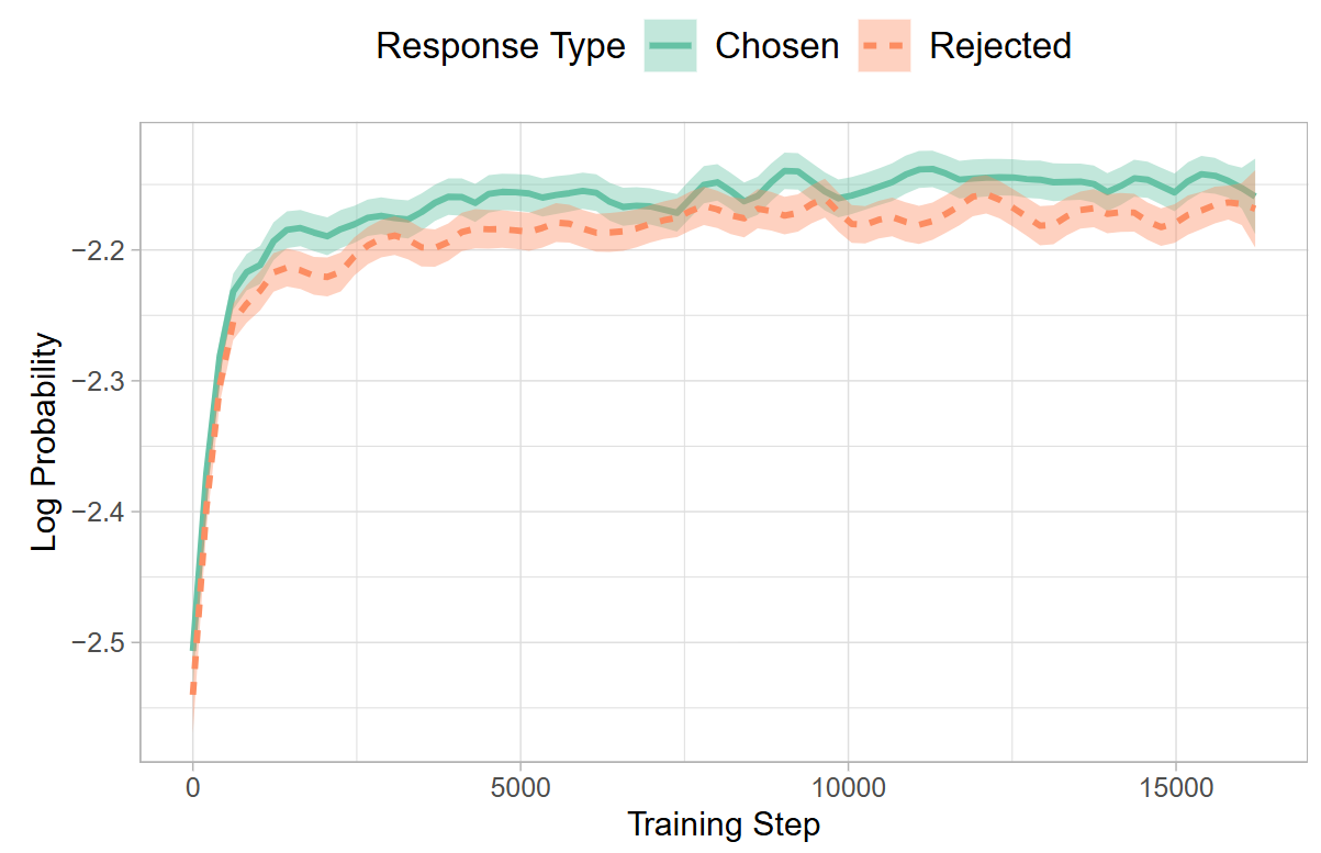
Fig. 13.1 Log probabilities for chosen and rejected responses during model fine-tuning on HH-RLHF dataset. Despite only chosen responses being used for SFT, rejected responses show a comparable likelihood of generation. Image from [HLT24].

Instead, we need a training methodology to explicitly reward the model when it is well-behaved and penalize the model when it is mis-behaved. Training the model to learn the human preference using rewards and penalities are the core of LLM alignment and preference learning. The pioneering approach is using reinforcement learning via the PPO algorithm [OWJ+22].

As shown in the Fig. 13.2, while SFT on instruction tuning dataset can improve model helpfulness and instruction following abilities, reinforcement learning can help the model achieve much larger gains than SFT.

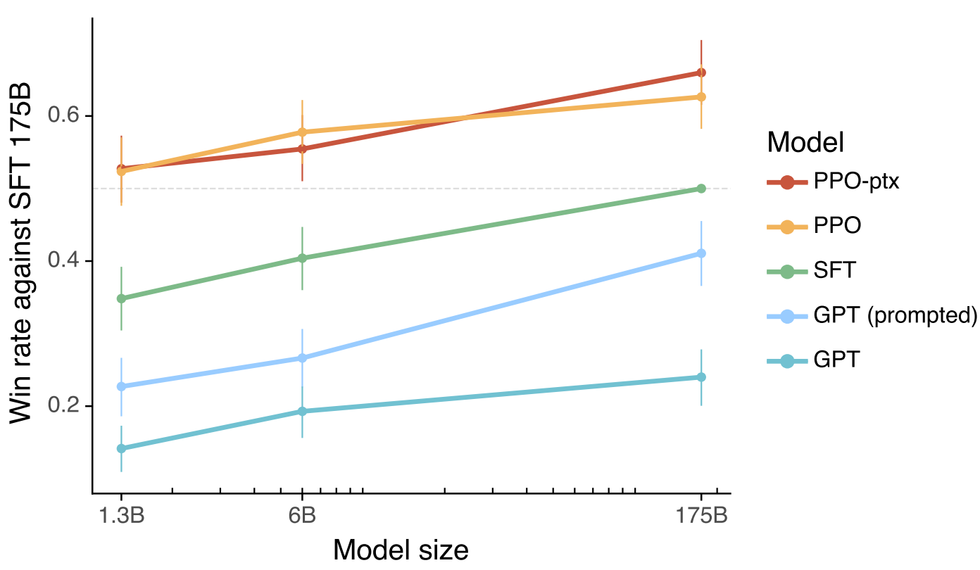
Fig. 13.2 Human evaluations of various models outputs show that how often outputs from each model were preferred to those from the 175B GPT-3 SFT model. The aligned models InstructGPT models (PPO-ptx) as well as variant (PPO) significantly outperform the GPT-3 baselines. Image from [OWJ+22].

13.2. Alignment Using RLHF

13.2.1. Overall methodology

The Alignment methodology [OWJ+22, SOW+20] has the following three steps [Fig. 13.3].

Step 1: SFT on demeonstration data: Collect demonstration data showing the target output given different prompt input, and SFT the model to mimic the target output.

Step 2: Preference/comparison labeling and reward modeling: Collect preference data, and train a reward model. The preference data set consists of labeler’s preferences towards different model outputs. Such preference data will be used to train a reward model to predict if human would prefer the model output given a model input.

Step 3 Optimize model generation policy with reward model: The reward model will be used to guide the model’s improvement on producing human preferred outputs. The optimization can be done using reinforcement learning, particularly the PPO algorithm [SWD+17].

Example 13.1 (Iterative reward model and policy improvement)

Steps 2 and 3 can be, and sometimes must be, iterated continuously; with model policy improved using reward model, the reward model might need be updated to further guide the improvement of the data. The reason is that

• The text generated from improved model will have a different distribution than what is used in reward model training.

• The trained reward model \(R_0\) is an approximate to the groundtruth reward model \(R_{GT}\). After one round of policy optimization, the model is likely overfitting to the \(R_0\), and actually performs poorly under the evaluation of \(R_{GT}\) (also see [SOW+20]).

To iterate the reward model to adapte to the new input distribution determined by the policy, we can collect more preference data, and combine with the original preference data to train a new RM and then a new policy.

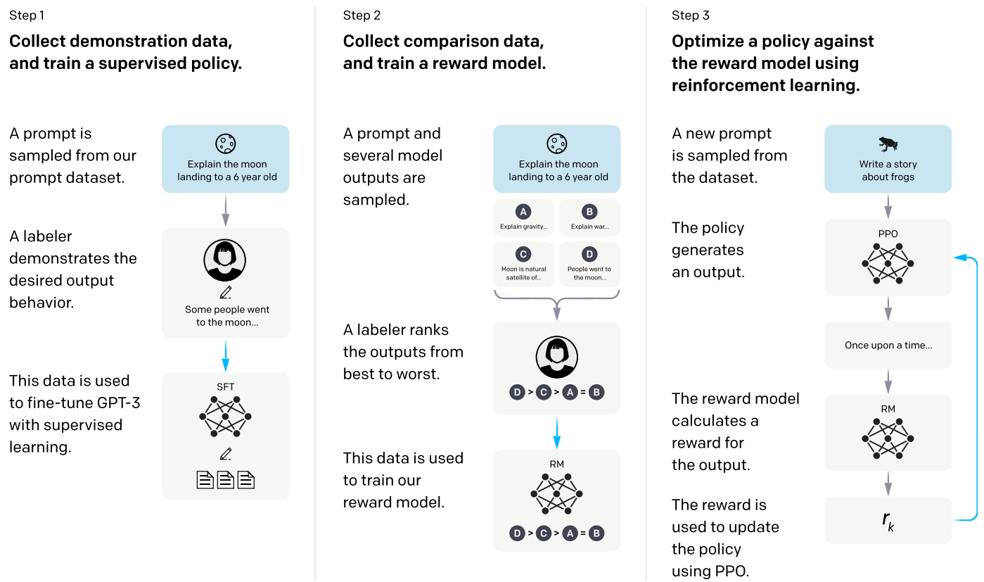
Fig. 13.3 A diagram illustrating the three steps of our method: (1) supervised fine-tuning (SFT), (2) reward model (RM) training, and (3) reinforcement learning via proximal policy optimization (PPO) on this reward model. Image from [OWJ+22].

Remark 13.1 (The importance of accurate reward model)

In classical RL, the reward model is usually deterministic and given. And RL algorithm optimizes the policy to maximize the reward. In LLM alignment, the reward model is not clearly defined and needs to be inferred from the preference data.

The size, quality, and distribution of the preference data affects how good we can train a reward model that approximates the ground-truth reward model. If there is a gap between the trained reward model and the ground-truth reward model, the gap will translate to the sub-optimality of the learned policy.

13.2.2. Preference Data and Reward Modeling

After SFT process on positive example, the trained model has improved ability on producing human preferred output. But it often has the overfitting risk and does not generalize well to unseen input data distributions. Preference data collections aims to provide both positive and negative examples, which are then used to train a reward model to help guide the model to generalize.

In the preference data collection process, human labelers assess different model outputs given the same prompt input and rank the output based on the human preference. The following table show the scoring standard used in the preference ranking process.

Table 13.1 How labeler evaluates the response quality

Metadata	Scale
Overall quality	Likert scale; 1-7
Fails to follow the correct instruction / task	Binary
Inappropriate for customer assistant	Binary
Hallucination	Binary
Satisifies constraint provided in the instruction	Binary
Contains sexual content	Binary
…	…

The objective of reward modeling is to train a model that take prompt \(x\) and one completion \(y\) as input and output a scalar score that align with human preference. More specificlly, let \(r(x, y)\) be the model’s scalar output, we have

\[r(x, y_w) > r(x, y_l) ~\text{if} ~ y_w \succ w_l\]

where \(y_w\) and \(y_l\) are two completions of prompt \(x\), and \(y_w\) is the preferred completion compared to \(y_l\).

Specifically, the loss function for the reward model (parameterized by \(\theta\)) is given by:

\[ L_\theta=-\frac{1}{\binom{K}{2}} E_{\left(x, y_w, y_l\right) \sim D}\left[\log \left(\sigma\left(r_\theta\left(x, y_w\right)-r_\theta\left(x, y_l\right)\right)\right)\right] \]

Here \(K\) (between 4 and 9) is the number reponses from the model for a given input, which forms \(\binom{K}{2}\) pairwise comparison for the labeler to rank. Usually, all completions associated with a model input are put into a single batch. This makes the training more efficient, as only one forward pass is needed, as well as helps model generation, as the model sees both positive and negative examples at the same time.

The interpretation of the loss function is that it encourages the reward model to give higher score to winning completions \(y_w\) then losing completions \(y_l\).

The reward model can be initialized from the SFT model (e.g., a 6B model) with the final embedding layer removed and a predictor head added on top to the final token’s last layer hidden dimensions. The reward model is trained to take in a prompt and response, and output a scalar reward.

13.2.3. Markov Decision Process (MDP) and Reinforcement learning

To understand how we can use a reward model to guide the improvement of the LLM using reinforcement learning, we can use the MDP framework. In the MDP fraemwork, we view model text generation as an agent’s sequential decision process. In particular, the MDP agent provides a response to the given prompt, need to decide the action (which token to generate) at each step. The alignment of LLM is equivalent to optimizing the agent on decision making policy to complete a final human preferred sequence.

Mathematically, an MDP is charcterized by tuple \(\langle\mathcal{S}, V, R, \pi, \gamma, T\rangle\).

• The initial state \(\boldsymbol{s}_0 \in \mathcal{S}\) is a task-specific prompt represented by \(\boldsymbol{x}=\left(x_0, \cdots, x_m\right)\). That is, \(\boldsymbol{s}_0 = \boldsymbol{x}\).

• An action in the environment \(a_t \in \mathcal{A}\) consists of a token from our vocabulary \(V\).

• The transition function or policy \(\pi: \mathcal{S} \times \mathcal{A} \rightarrow \mathcal{S}\) decides an action \(a_t\) and updatethe state \(s_{t-1}=\left(x_0, \cdots, x_m, a_0, \cdots, a_{t-1}\right)\).

• At the end of an episode a reward \(R: \mathcal{S} \rightarrow \mathbb{R}^1\) is provided by the reward model. The episode ends when the current time step \(t\) exceeds the horizon \(T\) or an end of sentence (EOS) token is generated.

Specifically, we will parameterize the step-wise policy by \(\theta\) such that a stochastic policy for each step is given by

\[\pi_s(a|s, \theta) = Pr(a_t = a| s_t = s, \theta).\]

13.2.4. The PPO Algorithm

PPO is a policy gradient algorithm used to find the optimal policy \(\pi^*\). We use the following notations:

• \((x, y)\) are prompt input \(x\) and completion \(y\) drawn from distribution \(D_{\pi}\) dependent on policy \(\pi\)

• \(\pi(y | x) \) is the trajectory level policy that connects to stepwise policy \(\pi_s (a | s)\) via

\[\pi(y | x) = \prod_{t <= T} \pi_s(y_t| y_{( < t)}, x).\]

We maximize the following objective function in the PPO RL training:

\[\begin{split} \begin{align*} &\max_{\phi}\operatorname{Objective}_{\text{PPO}}(\phi) \\ =& \max_{\phi} E_{(x, y) \sim D_{\pi_\phi^{\mathrm{RL}}}}\left[r_\theta(x, y)\right] - \operatorname{KL} (\pi_\phi^{\mathrm{RL}} || \pi_\phi^{\mathrm{SFT}}) \\ =& \max_{\phi} E_{(x, y) \sim D_{\pi_\phi^{\mathrm{RL}}}}\left[\underbrace{r_\theta(x, y)}_{\text{reward gain}}-\beta \underbrace{\log \pi_\phi^{\mathrm{RL}}(y \mid x) / \pi^{\mathrm{SFT}}(y \mid x)}_{\text{KL regularization}}\right] \end{align*} \end{split}\]

which contains the reward gain and KL regularization penality. Here \(\pi_\phi^{\mathrm{RL}}\) is the RL policy to be optimized, \(\pi^{\mathrm{SFT}}\) is the supervised trained model’s model as regularizer. The KL penality term aims to ensure that the optimized policy does not severely deviate from the original policy and overfit to the reward gain.

Besides the KL penality, to further prevent language modeling performance regression, we can add an auxillary objective to maximize the likelihood on texts sampled from pretraining datasets. The final objective, named PPO-ptx, is given by

\[ \operatorname{Objective}_{\text{PPO-ptx}}(\phi)= \operatorname{Objective}_{\text{PPO}}(\phi) + \gamma E_{x \sim D_{\text {pretrain }}}\left[\log \left(\pi_\phi^{\mathrm{RL}}(x)\right)\right] \]

where \(D_{\text {pretrain }}\) is the pretraining distribution.he pretraining loss coefficient, \(\gamma\), control the strength of the KL penalty and pretraining gradients respectively.

In Fig. 13.4, we illustrate the basic workflow of a PPO algorithm used to improve the langauge model. A more complete workflow is discussed in PPO Deep Dive.

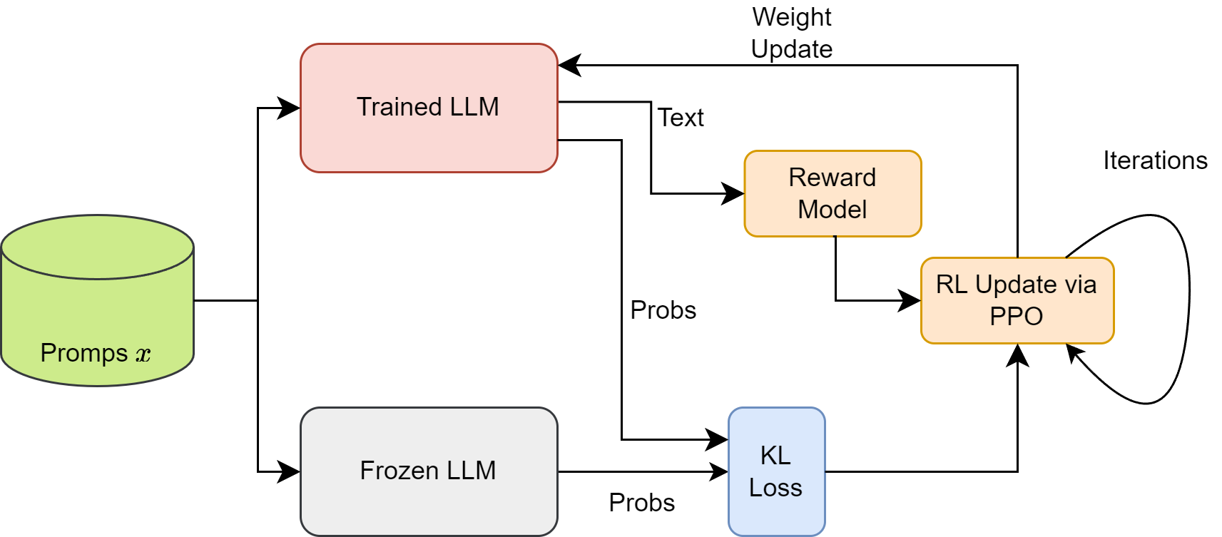
Fig. 13.4 Illustration of PPO based optimization, which uses a Frozen LLM and KL loss to prevent model optimization from going too far and reward model to encourge model to learn to generate highly-rewarded outputs.

Remark 13.2 (exploitation and exploration aspects from \(\gamma\))

\(\gamma\) controls the balance between exploitation and exploration. When \(\gamma \rightarrow 0\), the learning will concentrate on the max reward with full exploitation. When \(\gamma \rightarrow \infty\), optimal policy will be the same as \(\pi_{\mathrm{sft}}\) with full exploration.

13.2.5. PPO Deep Dive

Given the to-be-optimized poliy \(\pi(\phi)\) and a reference policy \(\pi_{ref}\), the objective function (to be maximized) used to update \(\pi\) is given by

\[ \operatorname{Objective}\left(\theta_{\phi}\right)=\min \left( r(y \mid x)A(s, a), \operatorname{Clip}\left(r(y \mid x), 1-\epsilon, 1+\epsilon\right) A(s, a)\right) \]

Here

• Here \(r(y \mid x)\) is the log probability ratio between \(\pi_\phi\) and \(\pi_{ref}\) on generating \(y\) given \(x\), which is given by

\[r(y \mid x) = \frac{\pi_\phi(y \mid x)}{\pi_{\theta_{ref}}(y \mid x)}\]

• \(\epsilon\) and the \(\operatorname{Clip}\) are acting to prevent \(\pi_\phi\) from going far away from \(\pi_{ref}\).

• \(A(y, x)\) is a scalar representing the advantage, in terms of reward, of \(y\) with respect to other possible \(y'\) under policy \(\pi_\phi\) (we will discuss it shortly).

The interpretation of the loss function is as follows:

• Advantage is positive: The objective function reduces to

\[ \operatorname{Objective}\left(\pi_\phi\right)=\min \left(r(y \mid x),(1+\epsilon)\right) A(s, a) \]

Because the advantage is positive, the objective will increase if the action \(y\) becomes more likely (i.e., if \(r(y \mid x) \) increases). Here the min says that if \(r(y \mid x) \) already above \(1 + \epsilon\), the policy will be not updated.

• Advantage is negative: The objective function reduces to

\[ \operatorname{Objective}\left(\pi_\phi\right)=\max \left(r(y \mid x),(1-\epsilon)\right) A(s, a) \]

Because the advantage is positive, the objective will improve if the action \(y\) becomes less likely (i.e., if \(r(y \mid x) \) decrease). Here the min says that if \(r(y \mid x) \) already below \(1 - \epsilon\), the policy will be not updated.

A typical implementation of PPO involves four models:

• An actor LLM (to be optimized) which specifies the generation policy.

• An frozen actor LLM, which specifies the reference policy.

• A reward model, which rate the final output \(y\) given prompt \(x\). Reward model is trained before the PPO.

• A value model, which estimates the expected reward at step \(t\) by following current policy. The input to the value model is \((y_{<t}, x)\).

Given an output \(y\) under current policy, the advantage of this output is given $\(A(y \mid x) = R(y \mid x) - V^{\pi}(x).\)$

A positive advantage indicates \(y\) is an output better than average output from current policy and is worth reinforced; a negative advantage indicates \(y\) is an output not better than the average, and it needs to be penalized. Note that the value function is a function of current policy, therefore it needs to be updated when the policy is updated.

There are other advanced methods to estimate more fine-grained level advantages on the token-level, as summarized in [ZDG+23].

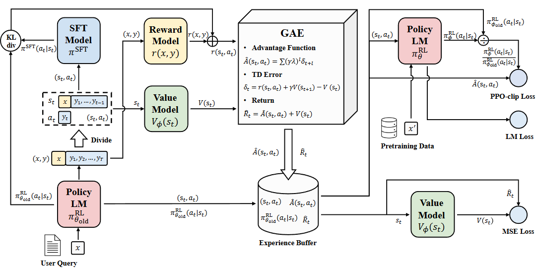
Fig. 13.5 Illustration of complete workflow PPO optimization. Image from [ZDG+23]

13.2.6. Discussion: SFT vs RLHF

SFT adopts a teacher-forcing approach, which directly optimizes the likelihood of a demonstration output. Such a token-level training way essentially does behavior cloning to imitate the demonstrations behavior.

On the other hand, RLHF firstly learns the reward model from preference data, and then employs it to improve the LLM with RL training (e.g., PPO). The reward model not just encourages positive behavior, but also discourages undesired responses.

In terms of generating comprehensive demonstration data vs preference labeling, preference labeling is much easier than writing the demonstration data.

RLHF essentially encourages LLMs to learn correct policies by contrasting the self-generated responses (discriminating between positive and negative responses). It not just forces the model to imitate external, positive only demonstration data but also forces the model to know when not to imitate or to know when to reject when there is uncertainty.

These negative penality signal can mitigate the hallucination or over-generalization issues associated with SFT on positive only data.

Example 13.2 (SFT on positive only data can lead to over-generalization)

Let’s consider how an LLM learns about geographic facts through SFT. During training, it might see examples like: Training Data:

Q: “What is the capital of France?”
A: “Paris is the capital of France.”
Q: “What is the capital of Germany?”
A: “Berlin is the capital of Germany.” \

The model learns a simple pattern: “[City] is the capital of [Country].” While this works for legitimate countries, it leads to problematic overgeneralization for fictional/hypothetical places:

Q: “What is the capital of Mars?”
A: “Olympus City is the capital of Mars.”

RLHF can mitigate the issue by introducing explicit examples of what not to do:

Question: “What is the capital of Mars?”
✓ Preferred: “Mars is a planet and does not have a capital city. While there are various geographic features on Mars, including Olympus Mons and Valles Marineris, the concept of a capital city applies to political entities on Earth.”
✗ Rejected: “Olympus Mons is the capital of Mars.”
✗ Rejected: “The Mars Colony Capital was established in 2020.”

Like classic RL algorithms, RLHF has the drawbacks like sample inefficiency, training complexity and instability. When adapted to LLMs, RLHF further relies on a strong SFT model as initial model checkpoint for efficiently achieving good performance

Overall, SFT is particularly useful to increase the model capacity of pre-trained model checkpoints right after pretraining, while RLHF is promising to further improve the model capacity of SFT models.

13.2.7. Discussion: Reward Model Criticality

For aligning LLM to human preference, reward modeling plays crucial role of human preferences and set the optimization direction for the model - if the reward model is built incorrectly or inaccruately, the model is optimized towards the wrong direction.

Let the groundtruth reward model be \(R_{GT}\). In reward modeling, we are training models \(R_0\) to approximate \(R_{GT}\). The typical reward modeling involves collecting preference label from labeler and build the reward model by learning from preference labels. The gap \(R_0\) and \(R_{GT}\) is affected by the following factors:

• The preference data quality, quantity, and distribution; more specifically,

  • label’s consistence with human preference

  • more high-quality preference data, the smaller the gap

  • the distribution should be broad and diverse to reflect the richness of the input space

• The model’s learning capacity - a weak model cannot capture intricate aspects of human preferences.

Suppose we obtain a reward model \(R_0\). What happen as we optimizes the model policy towards the reward model? Optimizing against reward model \(R_0\) is supposed to make our policy align with human preferences, i.e., \(R_{GT}\). But the \(R_0\) is not a perfect representation of our labeler preferences, as it has limited capacity and only sees a limited amount of preference data from a likely narrow distribution of inputs. Studies from [GSH23, SOW+20] show that optimizing towards an imperfect reward model can run into the overfitting risk, leading to a model achieving high score with respect to \(R_0\) but actually low score with respect to \(R_{GT}\) [Fig. 13.6]. To minimize the gap between \(R_0\) and \(R_{GT}\), they also empirically show that one can enlarge the model size as well as the training data size.

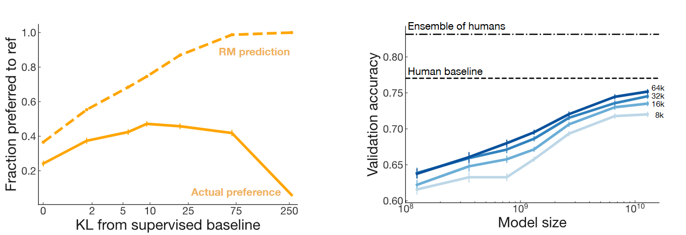
Fig. 13.6 (Left) The overfitting phenomonon of optimizing the model towards an imperfect reward model, leading to a model achieving high score with respect to \(R_0\) (dash line) but actually low score with respect to \(R_{GT}\) (solid line). Here the KL distance w.r.t. the initial policy is used to measure the degree of over-optimization. (Right) To reduce the gap to \(R_{GT}\), one can enlarge model size as well as enlarge preference training data.

Studies from [WZC+24] further reveals that

• The importance of label quality - incorrect and ambiguous preference pairs in the dataset may hinder the reward model from accurately capturing human intent.

• Poor generation of reward model - reward models trained on data from a specific distribution often struggle to generalize to examples outside that distribution and are not suitable for iterative RLHF training.

To mitigate these drawbacks, they proposed that

• One can measure the strength of preferences within the data using ensemble reward models.

• Use labeling smoothing to reduce the impact of noisy labels (also discussed in Smoothing preference label).

• Use adaptive margin, originated from contrastive learning, in training reward model (also discussed in Simple DPO).

13.3. RL Variants

13.3.1. Group Relative Policy Optimization (GRPO)

DeepSeek team [SWZ+24] proposed a modified PPO, known as GRPO, to reduce the computation cost and improve the value function estimation for the original PPO algorithm. As shown in shao2024deepseekmath, GRPO does not need an additional value model; baseline score for advantage computation is directly estimated from group scores, significantly reducing training resources.

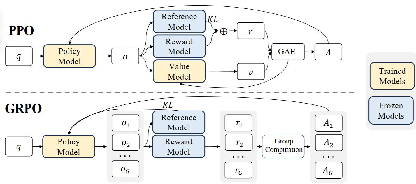
Fig. 13.7 Comparison of PPO and GRPO. GRPO does not need an additional value model; baseline score for advantage computation is directly estimated from group scores, significantly reducing training resources. Image from [SWZ+24]

More specifically, the loss function of GRPO is given by

(13.1)\[\mathcal{J}_{G R P O}(\theta)=\mathbb{E}_{q \sim P(Q),\left\{o_i\right\}_{i=1}^G \sim \pi_{\theta_{o l d}}(O \mid q)} \left[ \frac{1}{G} \sum_{i=1}^G \frac{1}{\left|o_i\right|} \sum_{t=1}^{\left|o_i\right|}\left(\min \left[r_{i,t} \hat{A}_{i, t}, \operatorname{clip}\left(r_{i,t}, 1-\varepsilon, 1+\varepsilon\right) \hat{A}_{i, t}\right]-\beta \mathbb{D}_{K L}\left[\pi_\theta| | \pi_{r e f}\right]\right)\right] \]

Here

• Question \(q\) is sampled from distribution \(P(Q)\); \(G\) output \(\left\{o_i\right\}\) are sampled from the old policy \(\pi_{\theta_{o l d}}(O \mid q)\).

• \(r_{i,t}\) is the log probability ratio for output \(i\) at step \(t\), which is given by

\[r_{i,t} = \frac{\pi_\theta\left(o_{i, t} \mid q, o_{i,<t}\right)}{\pi_{\theta_{o l d}}\left(o_{i, t} \mid q, o_{i,<t}\right)}\]

• \(\hat{A}_{i, t}\) is the group-estiamted advantage based on reward model \(R\) for output \(i\) at step \(t\).

  1. If the reward model is an outcome reward model that provides rewards only at the end of the each output \(o_t\), then

\[\hat{A}_{i, t}= \hat{A}_{i} = \frac{R_{i}-\operatorname{mean}\left(\left\{R_{1}, R_{2}, \cdots, r_{G}\right\}\right)}{\operatorname{std}\left(\left\{R_{1}, R_{2}, \cdots, r_{G}\right\}\right)}\]

2. If the reward model is a process reward model that provides token-level rewards, then

\[\hat{A}_{i, t}=\frac{R_{i,t}-\operatorname{mean}\left(\left\{R_{1,t}, R_{2,t}, \cdots, r_{G,t}\right\}\right)}{\operatorname{std}\left(\left\{R_{1,t}, R_{2,t}, \cdots, r_{G,t}\right\}\right)}\]

• The computation of KL divergence is based on an modified low-variance unbiased estimator

\[\mathbb{D}_{K L}\left[\pi_\theta| | \pi_{r e f}\right]_{i,t}=\frac{\pi_{r e f}\left(o_{i, t} \mid q, o_{i,<t}\right)}{\pi_\theta\left(o_{i, t} \mid q, o_{i,<t}\right)}-\log \frac{\pi_{r e f}\left(o_{i, t} \mid q, o_{i,<t}\right)}{\pi_\theta\left(o_{i, t} \mid q, o_{i,<t}\right)}-1\]

When estimating advantages, GRPO directly use sample uses the average reward of multiple sampled outputs, produced in response to the same question, as the baseline.

Removing value function has critical benefits:

• The value function employed in PPO is typically another model of comparable size as the policy model - training the value function itself brings a substantial computational burden

• In the LLM context, usually only the last token is assigned a reward score by the reward model, such sparse reward also presents challenge to train an accurate value function.

We summarize the GRPO algorithm in the following.

Algorithm 13.1 (Iterative Group Relative Policy Optimization)

Input: Initial policy model \(\pi_{\text{init}}\); reward models \(R\); task prompts \(\mathcal{D}\); Reward model iteration \(I\), number of batches \(M\), and gradient steps \(\mu\).

Output: \(\pi_{\theta}\)

1. Initialize policy model \(\pi_{\theta} \leftarrow \pi_{\text{init}}\)

2. For iteration = 1, …, \(I\) do

   1. Set reference model \(\pi_{\text{ref}} \leftarrow \pi_{\theta}\)

   2. For step = 1, …, \(M\) do

      1. Sample a batch of tasks \(\mathcal{D}_b\) from \(\mathcal{D}\)

      2. Update the old policy model \(\pi_{\text{old}} \leftarrow \pi_{\theta}\)

      3. Sample \(G\) outputs \(\{o_i\}_{i=1}^{G} \sim \pi_{\theta}(\cdot | q) \) for each question \( q \in \mathcal{D}_b \)

      4. Compute rewards for each \(o_i\)

      5. Compute \(\hat{A_{i,t}}\) for the \(t\)-th token of \(o_i\) through group relative advantage estimation.

      6. For GRPO iteration = 1, …, ( J ) do

         1. Update the policy model ( \pi_{\theta} ) by maximizing the GRPO objective {eq}``

   3. Update reward model \(R\) through continuous training using a replay mechanism.

13.4. DPO

13.4.1. Overview

DPO (Direct Preference Optimization) [RSM+24] improves the classical RLHF-PPO algorithm from the following two aspects:

• Additional reward model is no longer need; Instead, the LLM itself can act as a reward model itself; preference data is directly used to train an aligned model in one step.

• Reinforcement learning no longer need. Optimizing the policy of an LLM towards a reward model is mathematially equivalent to directly training the LLM as a reward model on the preference data.

The following illustrates from the DPO paper to visually compare the differences between RLHF-PPO and DPO

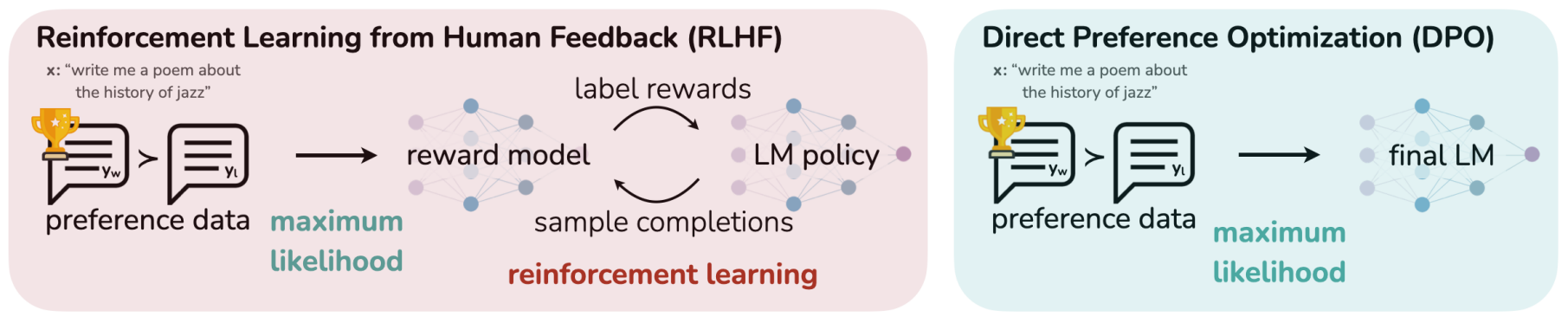
Fig. 13.8 DPO optimizes for human preferences while avoiding reinforcement learning. Existing methods for fine-tuning language models with human feedback first fit a reward model to a dataset of prompts and human preferences over pairs of responses, and then use RL to find a policy that maximizes the learned reward. In contrast, DPO directly optimizes for the policy best satisfying the preferences with a simple classification objective. Image from [RSM+24].

The DPO training pipelines consists of the following two steps:

• Preference data construction - sample completions \(y_1, y_2 \sim \pi_{\text {ref }}(\cdot \mid x)\) for every prompt \(x\), label with human preferences to construct the offline dataset of preferences \(\mathcal{D}=\left\{x^{(i)}, y_w^{(i)}, y_l^{(i)}\right\}_{i=1}^N\)

• Optimize the language model as a reward model, which is equivalent to optimize \(\pi_\theta\) to minimize \(\mathcal{L}_{\mathrm{DPO}}\) for the given \(\pi_{\text {ref }}\) and \(\mathcal{D}\) and desired \(\beta\).

\[ \mathcal{L}_{\mathrm{DPO}}\left(\pi_\theta ; \pi_{\mathrm{ref}}\right)=-\mathbb{E}_{\left(x, y_w, y_l\right) \sim \mathcal{D}}\left[\log \sigma\left(\beta \log \frac{\pi_\theta\left(y_w \mid x\right)}{\pi_{\mathrm{ref}}\left(y_w \mid x\right)}-\beta \log \frac{\pi_\theta\left(y_l \mid x\right)}{\pi_{\mathrm{ref}}\left(y_l \mid x\right)}\right)\right]. \]

Note: Since the preference datasets are sampled using \(\pi^{\mathrm{SFT}}\), we initialize \(\pi_{\text {ref }}=\pi^{\mathrm{SFT}}\) whenever available.

13.4.2. Preliminary: Preference modeling

The Bradley-Terry model [BT52] is a probability model for the outcome of pairwise comparisons between items, teams, or objects. Given a pair of items \(i\) and \(j\) drawn from some population, it estimates the probability that the pairwise comparison \(i>j\) turns out true, as

\[ \operatorname{Pr}(i\succ j)=\frac{s_i}{s_i+s_j} \]

where \(s_i\) is a positive real-valued score assigned to individual \(i\).

\[ P\left(y_1 \succ y_2 \mid x\right)=\frac{\exp \left[r\left(x, y_1\right)\right]}{\exp \left[r\left(x, y_1\right)\right]+\exp \left[r\left(x, y_2\right)\right]}\]

Remark 13.3 (Relationship to logistic regression)

\[\operatorname{logit} \operatorname{Pr}(i>j)=\log \frac{\operatorname{Pr}(i>j)}{1-\operatorname{Pr}(i>j)}=\log \frac{\operatorname{Pr}(i>j)}{\operatorname{Pr}(j>i)}=\beta_i-\beta_j \]

13.4.3. Driving the DPO

Here we outline the key steps to derive the DPO objective function, and explain why optimizing LLM as a reward model is equivalent to optimizing its policy.

First we start with the objective of LLM alignment with a given fixed reward function \(r\) with a KL constraint,

\[ \max_\pi \mathbb{E}_{x, y \sim \mathcal{D}_{\pi}}[r(x, y)]-\beta \mathbb{D}_{\mathrm{KL}}\left[\pi(y \mid x) \| \pi_{\text {ref }}(y \mid x)\right]. \]

It turns out that we can obtain the theoretical solution of \(\pi_r(y|x)\) given by

\[\pi_r(y|x) = \frac{1}{Z(x)}\pi_{\text{ref}}(y|x) \exp(\frac{1}{\beta}r(x, y)),\]

where \(Z(x)\) is partition funciton dependent only on \(x\) and \(\pi_{\text{ref}}\), which is given by \(Z(x)=\sum_y \pi_{\mathrm{ref}}(y \mid x) \exp \left(\frac{1}{\beta} r(x, y)\right)\).

With some algebra, we can also represent the reward funciton with \(\pi_r(y|x)\), given by

\[r(x, y) = \beta \log \frac{\pi_r (y|x)}{\pi_{\text{ref}}(y|x)} + \beta \log Z.\]

Remark 13.4 (Implicit reward)

Note that here the reward can be interpreted as the log ratio of the likelihood of a response between the current policy model and the reference model. And the policy is the maximizer of the objective function given the reward.

Note that we have just shown that that reward function \(r(x, y)\) and its corresponding optimal policy \(\pi_{\text{ref}}(y|x)\) are inter-convertable, with a funciton \(Z(x)\) independent of \(y\).

This means that instead of numerically optimizing policy \(\pi\), we can also choose optimize the reward function. When the reward function is optimized, the policy is also optimized at the same time (in other words, we can analytically solve the optimal policy).

Given the available preference data, one formulation to optimize the reward function is the Bradley-Terry (BT) objective, that is

\[\mathcal{L}_{BT} = -\mathbb{E}_{\left(x, y_w, y_l\right) \sim \mathcal{D}}\left[\log \sigma (r(y_w, x) - r(r_l, x)) \right].\]

By leveraging the relationship between reward \(r\) and policy \(\pi\), we can arrive at the DPO loss function:

\[ \mathcal{L}_{\mathrm{DPO}}\left(\pi_\theta ; \pi_{\mathrm{ref}}\right)=-\mathbb{E}_{\left(x, y_w, y_l\right) \sim \mathcal{D}}\left[\log \sigma\left(\beta \log \frac{\pi_\theta\left(y_w \mid x\right)}{\pi_{\mathrm{ref}}\left(y_w \mid x\right)}-\beta \log \frac{\pi_\theta\left(y_l \mid x\right)}{\pi_{\mathrm{ref}}\left(y_l \mid x\right)}\right)\right]. \]

where the terms \(\beta \log Z\) are canceled during subtraction.

Remark 13.5 (How DPO loss work)

The gradient of DPO loss function is given by:

\[\nabla_\theta \mathcal{L}_{\mathrm{DPO}}\left(\theta, y_w, y_l\right)=-\left(1-\hat{p}_\theta\right) [\underbrace{\nabla_\theta \log \pi_\theta\left(y_w\right)}_{\text {upweight } y_w}-\underbrace{\nabla_\theta \log \pi_\theta\left(y_l\right)}_{\text {downweight } y_l}] \]

where for the preference completion pair \(y_w \succ y_l\), as long as \(\hat{p} < 1\), there will gradients to upweight the probability of generating \(y_w\) and downweight the probability of generating \(y_l\).

Remark 13.6 (Monitor DPO training process)

The DPO algorithm aims to make winning responses have higher probability and losing responses have lower probability. If the training works as expected, beside the overall loss is descreasing, we will see

• \(\log \frac{\pi_\theta\left(y_w \mid x\right)}{\pi_{\mathrm{ref}}\left(y_w \mid x\right)}\) becomes larger for the same \(y_w\).

• \(\log \frac{\pi_\theta\left(y_l \mid x\right)}{\pi_{\mathrm{ref}}\left(y_l \mid x\right)}\) becomes smaller for the same \(y_l\).

13.4.4. Discussion: DPO vs RL

DPO and RL-PPO have the same objective - optimizing LLM’s generation behavior towards what human prefer. Since there is no theorectially correct human preference model \(R_{GT} \)available; instead of, we use colect preference label data \(D\) from human labelers to reflect what human prefer.

In the RL-PPO approach, a proxy reward model \(R_0\) is first learned from human-labeled data to approximate \(R_{GT}\); then the PPO algorithm is used to optimize the model policy toward \(R_0\), with the hope that optimizing towards \(R_0\) will more or less optimizing towards \(R_{GT}\). As a comparison, instead of learning a reward model, DPO directly optimizes the policy over preference data.

Normally, the finite-sized \(D\) cannot cover the whole input-output space, and the proxy reward model \(R_0\) often performs poorly in the face of out-ofdistribution data [Also see Discussion: Reward Model Criticality]. Studies from [XFG+24] show that with an imperfect reward model, the policy \(\pi_{\text{DPO}}\) from DPO, which is trained to maximize \(y_w\) and minimize \(y_l\) probability, can unexpectedly favor out of distribution responses (i.e., output \(y\) that is different from \(y_w\) and \(y_l\) ) and lead to unpredictable behaviors.

The reason for the lack of robustness for DPO compared to RL-PPO is that

• DPO is learning from limited, offline generated preference data and there is no additional exploration of the input output space during training. The resulting model has a hard time to generate well beyond what is included in the preference data. In the loss function, this is a limited regularization effect on \(\pi_{\text{DPO}}(y)\), when \(y\) is largely different from \(y_w\) or \(y_l\) in the training data.

• RL-PPO is online learning with exploration. After obtaining the reward model, RL-PPO does not need offline generated data to train the policy \(\pi_{\text{PPO}}\); the LLM agent itself generates outputs and learn from the reward signal from reward model. The self-generation approach enables RL to have in theory unlimited amount of data to cover much large ranges of input and output distributions. Even an output \(y\) is largely different from \(y_w\) or \(y_l\) in the training data, such \(y\) might be covered in the online exploration process; As a result, at least the KL regularization in the loss function can still properly guide \(\pi_{\text{PPO}}(y)\) to not to be far away from \(\pi_{\text{ref}}(y)\).

Nevertheless, from reward modeling perspective, DPO and RL-PPO share the vulnerbility to reward model

• Both DPO and RL-PPO is approximating the ground-truth reward model using limited, offline generated preference data. The size and distribution of preference data affect the gap of trained reward model and the ground-truth reward model. The gap in the reward model will translate to the gap of policy.

• To overcome the limitation of reward modeling on offline generated data, we can use iterative approach to improve reward modeling (i.e., collecting additional preference data label on DPO or RL-PPO policies for continous reward modeling improvement).

Remark 13.7 (Effective implementing PPO is critical)

Although RL-PPO has better robustness to imperfect reward model [XFG+24], an effective implementation of PPO is critical. This involves tricks like advantage normalization, large batch size, and exponential moving average update for the reference model, etc.

13.4.5. Iterative DPO

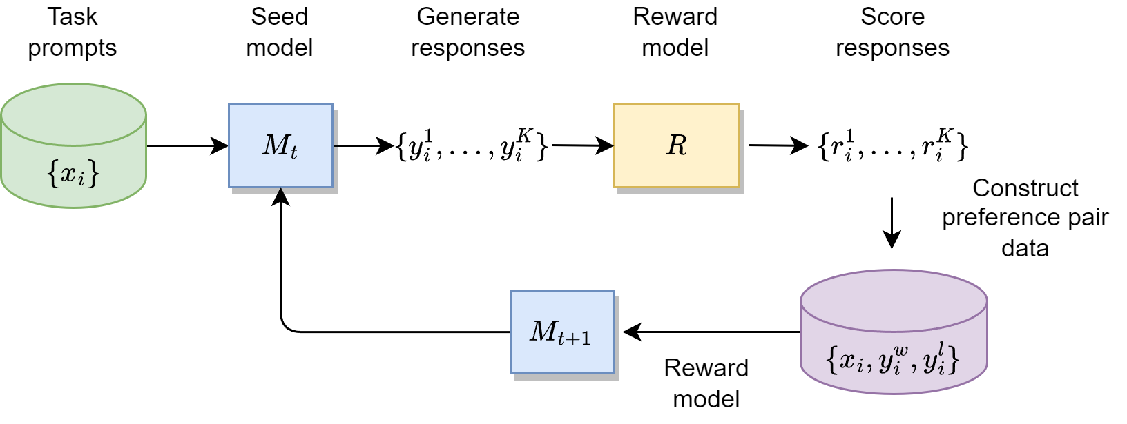
DPO can also be used iteratively (e.g., 3-5 iterations)to enhance the alignment results. As shown in Fig. 13.9,

• Starting with a SFT model checkpoint \(M_0\), one can go through the DPO data annotation and training process to arrive at \(M_1\)

• Preference pair data will be collected from \(M_1\) and used to train \(M_2\).

Iterative DPO has demonstrated its effectiveness in different scenarios [PYC+24, DJP+24, TMS+3b, CDY+24, YPC+24].

Fig. 13.9 Workflow of iterative DPO Image from [RSM+24].

13.5. DPO Variants

13.5.1. Smoothing preference label

When the preference label is noisy (e.g., annotation error/noise), a more robust DPO approach is desired [Mit23]. It assumes that the labels have been flipped with some small probability \(\epsilon \in(0,0.5)\). We can use a conservative target distribution instead, \(p\left(y_w \succ y_l\right)=1-\epsilon\), giving BCE loss:

\[\begin{split} \begin{aligned} \mathcal{L}_{\mathrm{DPO}}^\epsilon\left(\theta, y_w, y_l\right) & =-(1-\epsilon) \log \hat{p}_\theta\left(y_w \succ y_l\right)-\epsilon \log \left(1-\hat{p}_\theta\left(y_w \succ y_l\right)\right) \\ & =(1-\epsilon) \mathcal{L}_{\mathrm{DPO}}\left(\theta, y_w, y_l\right)+\epsilon \mathcal{L}_{\mathrm{DPO}}\left(\theta, y_l, y_w\right) \end{aligned} \end{split}\]

The gradient of \(\mathcal{L}_{\mathrm{DPO}}^\epsilon\left(\theta, y_w, y_l\right)\) is reduced to the simplified form :

\[\begin{split} \begin{aligned} \nabla_\theta \mathcal{L}_{\mathrm{DPO}}^\epsilon\left(\theta, y_w, y_l\right) & =-\left((1-\epsilon)\left(1-\hat{p}_\theta\right)-\epsilon \hat{p}_\theta\right)[\underbrace{\nabla_\theta \log \pi_\theta\left(y_w\right)}_{\text {upweight } y_w}-\underbrace{\nabla_\theta \log \pi_\theta\left(y_l\right)}_{\text {downweight } y_l}] \\ & =\quad\left(\hat{p}_\theta-(1-\epsilon)\right)\left[\nabla_\theta \log \pi_\theta\left(y_w\right)-\nabla_\theta \log \pi_\theta\left(y_l\right)\right] \end{aligned} \end{split}\]

13.5.2. Simple DPO

The simple DPO[MXC24] improve the original DPO from two aspects:

• Make the sequence likelihood function used in implicit reward be aligned with the likelihood of actual sequence decoding.

• Add a margin to encourage larger reward gap between positive sequence and negative sequence, which will help generalzation.

First, the authors argue that original DPO derives the closed form implicit reward as the log ratio of the likelihood of a response between the current policy model and the reference model plus a constant only depending on \(x\)

\[r(x, y)=\beta \log \frac{\pi_\theta(y \mid x)}{\pi_{\mathrm{ref}}(y \mid x)} + Const(x).\]

In actual decoding process, the likelihood of a response is usually length averaged (see Beam search decoding), for example,

\[p_\theta(y \mid x)=\frac{1}{|y|} \log \pi_\theta(y \mid x)=\frac{1}{|y|} \sum_{i=1}^{|y|} \log \pi_\theta\left(y_i \mid x, y_{<i}\right)\]

Naturally, we consider replacing the reward formulation in DPO with \(p_\theta\) above, so that it aligns with the likehood metric that guides generation. This results in a length-normalized reward:

\[ r_{\mathrm{SimPO}}(x, y)=\frac{\beta}{|y|} \log \pi_\theta(y \mid x)=\frac{\beta}{|y|} \sum_{i=1}^{|y|} \log \pi_\theta\left(y_i \mid x, y_{<i}\right) \]

The author argues that normalizing the reward with response lengths is crucial: removing the length normalization term from the reward formulation results in a bias toward generating longer but lower-quality sequences.

Additionally,a target reward margin term, \(\gamma>0\), is added to the Bradley-Terry objective to ensure that the reward for the winning response, \(r\left(x, y_w\right)\), exceeds the reward for the losing response, \(r\left(x, y_l\right)\), by at least \(\gamma\). This is margin idea is also commonly used in constrastive learning.

\[ p\left(y_w \succ y_l \mid x\right)=\sigma\left(r\left(x, y_w\right)-r\left(x, y_l\right)-\gamma\right) \]

Combined these ideas together, we arrive at the SimPO loss function:

\[ \mathcal{L}_{\operatorname{SimPO}}\left(\pi_\theta\right)= -\mathbb{E}\left[\log \sigma\left(\frac{\beta}{\left|y_w\right|} \log \pi_\theta\left(y_w \mid x\right)-\frac{\beta}{\left|y_l\right|} \log \pi_\theta\left(y_l \mid x\right)-\gamma\right)\right] \]

Note that, unlike the traditional DPO, SimPO does not require a reference model, making it more lightweight and easier to implement.

13.5.3. DPO-Positive and Regularized DPO

DPO and its variant usually perform well when the preference paired data consists of strong contrastive pairs, i.e., positive example and negative example are sharply different from edit distance perspective. For these examples, DPO can enhance the probability of generating the positive and reduce the probability of generating the negative.

However, for paired data that is small edit distance (i.e., positive and negative pairs look similiar), DPO algorithm can lead to failure mode - that is, both the generating probability of positive and negative example decrease (although negative ones decrease more).

Authors from [PKD+24] not only provides an theoretical understanding of above phenomonon, they will propose one approach to mitigate the failure mode, known as DPO-Positive or DPO-P.

The key idea is to add a penality term when the model reduces the probability of positive examples. The modified loss function is given by

\[\begin{split} \mathcal{L}_{\mathrm{DPOP}}\left(\pi_\theta\right)=-\mathbb{E}_{\left(x, y_w, y_l\right) \sim D}\left[\log \sigma \left(\beta \left(\log \frac{\pi_\theta\left(y_w \mid x\right)}{\pi_{\mathrm{ref}}\left(y_w \mid x\right)}\right.\right.\right. -\log \frac{\pi_\theta\left(y_l \mid x\right)}{\pi_{\mathrm{ref}}\left(y_l \mid x\right)} \\ \left.\left.\left.-\lambda \cdot \max \left(0, \log \frac{\pi_{\mathrm{ref}}\left(y_w \mid x\right)}{\pi_\theta\left(y_w \mid x\right)}\right)\right)\right)\right] \end{split}\]

where \(\lambda>0\) is a hyperparameter determining the strength of the penalty. From the Bradley-Terry modeling framework,

• for the negative \(y_l\), the loss function is encourging minimize term of

\[ \beta \cdot \log \frac{\pi_\theta(y_l \mid x)}{\pi_{\mathrm{ref}}(y_l \mid x)} \]

• for the positive \(y_w\), the loss function is encouraging maximizing the term of

\[\beta\left[\log \frac{\pi_\theta\left(y_w \mid x\right)}{\pi_{\mathrm{ref}}(y_w \mid x)}-\lambda \cdot \max \left(0, \log \frac{\pi_{\mathrm{ref}}(y_w \mid x)}{\pi_\theta(y_w \mid x)}\right)\right]. \]

Clearly, if we want to maximize these terms for \(y_w\), we need to ensure that the generating probability \(\pi_{\theta}(y_w|x)\) not to reduce too much from \(\pi_{\text{ref}}(y_w|x)\).

On a similar line of thinking, [PYC+24] proposed using the negative log likelihood (NLL) loss as a regularizer, which gives the following loss function:

\[ \mathcal{L}_{\mathrm{DPO-R}}\left(\pi_\theta\right)=-\mathbb{E}_{\left(x, y_w, y_l\right) \sim D}\left[\log \sigma \left(\beta \left(\log \frac{\pi_\theta\left(y_w \mid x\right)}{\pi_{\mathrm{ref}}\left(y_w \mid x\right)} -\log \frac{\pi_\theta\left(y_l \mid x\right)}{\pi_{\mathrm{ref}}\left(y_l \mid x\right)}\right)\right) + \frac{\lambda}{|y_w|}\log\left(\pi_\theta(y_w|x)\right) \right] \]

The authors found that in reasoning tasks, having the NLL loss regularization is critical to promote the likelihood of positive (chosen) sequences [Fig. 13.10].

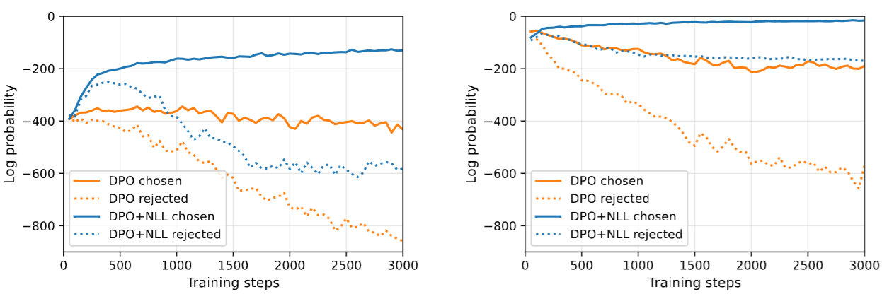
Fig. 13.10 Effect on NLL regularizer loss on applying DPO in reasoning tasks. (left) Without regularizer loss, the likelihood of chosen sequences is decreasing when the model is initialized from Llama (left) and a positive-example FT checkpoint (right). After FT, the decreasing of the likelihood is more severe. Image from [PYC+24].

13.5.4. Cringe Loss

[AGX+22, XLSW23]

13.6. Bibliography

[AGX+22]

Leonard Adolphs, Tianyu Gao, Jing Xu, Kurt Shuster, Sainbayar Sukhbaatar, and Jason Weston. The cringe loss: learning what language not to model. arXiv preprint arXiv:2211.05826, 2022.

[BKK+22]

Yuntao Bai, Saurav Kadavath, Sandipan Kundu, Amanda Askell, Jackson Kernion, Andy Jones, Anna Chen, Anna Goldie, Azalia Mirhoseini, Cameron McKinnon, and et al. Constitutional AI: harmlessness from AI feedback. ArXiv:2212.08073, 2022.

[BT52]

Ralph Allan Bradley and Milton E. Terry. Rank analysis of incomplete block designs: i. the method of paired comparisons. Biometrika, 39(3/4):324–345, 1952. URL: http://www.jstor.org/stable/2334029 (visited on 2024-09-20).

[CDY+24]

Zixiang Chen, Yihe Deng, Huizhuo Yuan, Kaixuan Ji, and Quanquan Gu. Self-play fine-tuning converts weak language models to strong language models. arXiv preprint arXiv:2401.01335, 2024.

[DJP+24]

Abhimanyu Dubey, Abhinav Jauhri, Abhinav Pandey, Abhishek Kadian, Ahmad Al-Dahle, Aiesha Letman, Akhil Mathur, Alan Schelten, Amy Yang, Angela Fan, and others. The llama 3 herd of models. arXiv preprint arXiv:2407.21783, 2024.

[GSH23]

Leo Gao, John Schulman, and Jacob Hilton. Scaling laws for reward model overoptimization. In International Conference on Machine Learning, 10835–10866. PMLR, 2023.

[HLT24]

Jiwoo Hong, Noah Lee, and James Thorne. Reference-free monolithic preference optimization with odds ratio. arXiv e-prints, pages arXiv–2403, 2024.

[MXC24]

Yu Meng, Mengzhou Xia, and Danqi Chen. Simpo: simple preference optimization with a reference-free reward. 2024. URL: https://arxiv.org/abs/2405.14734, arXiv:2405.14734.

[Mit23]

Eric Mitchell. A note on dpo with noisy preferences & relationship to ipo. 2023. URL: https://ericmitchell.ai/cdpo.pdf.

[OWJ+22] (1,2,3,4)

Long Ouyang, Jeff Wu, Xu Jiang, Diogo Almeida, Carroll L. Wainwright, Pamela Mishkin, Chong Zhang, Sandhini Agarwal, Katarina Slama, Alex Ray, John Schulman, Jacob Hilton, Fraser Kelton, Luke Miller, Maddie Simens, Amanda Askell, Peter Welinder, Paul Christiano, Jan Leike, and Ryan Lowe. Training language models to follow instructions with human feedback. 2022. URL: https://arxiv.org/abs/2203.02155, arXiv:2203.02155.

[PKD+24]

Arka Pal, Deep Karkhanis, Samuel Dooley, Manley Roberts, Siddartha Naidu, and Colin White. Smaug: fixing failure modes of preference optimisation with dpo-positive. arXiv preprint arXiv:2402.13228, 2024.

[PYC+24] (1,2,3)

Richard Yuanzhe Pang, Weizhe Yuan, Kyunghyun Cho, He He, Sainbayar Sukhbaatar, and Jason Weston. Iterative reasoning preference optimization. arXiv preprint arXiv:2404.19733, 2024.

[RSM+24] (1,2,3)

Rafael Rafailov, Archit Sharma, Eric Mitchell, Stefano Ermon, Christopher D. Manning, and Chelsea Finn. Direct preference optimization: your language model is secretly a reward model. 2024. URL: https://arxiv.org/abs/2305.18290, arXiv:2305.18290.

[SWD+17]

John Schulman, Filip Wolski, Prafulla Dhariwal, Alec Radford, and Oleg Klimov. Proximal policy optimization algorithms. 2017. URL: https://arxiv.org/abs/1707.06347, arXiv:1707.06347.

[SWZ+24] (1,2)

Zhihong Shao, Peiyi Wang, Qihao Zhu, Runxin Xu, Junxiao Song, Xiao Bi, Haowei Zhang, Mingchuan Zhang, YK Li, Y Wu, and others. Deepseekmath: pushing the limits of mathematical reasoning in open language models. arXiv preprint arXiv:2402.03300, 2024.

[SOW+20] (1,2,3)

Nisan Stiennon, Long Ouyang, Jeffrey Wu, Daniel Ziegler, Ryan Lowe, Chelsea Voss, Alec Radford, Dario Amodei, and Paul F Christiano. Learning to summarize with human feedback. Advances in Neural Information Processing Systems, 33:3008–3021, 2020.

[TMS+3b]

Hugo Touvron, Louis Martin, Kevin Stone, Peter Albert, Amjad Almahairi, Yasmine Babaei, Nikolay Bashlykov, Soumya Batra, Prajjwal Bhargava, Shruti Bhosale, and et al. LLaMA 2: open foundation and fine-tuned chat models. ArXiv:2307.09288, 2023b.

[WZC+24]

Binghai Wang, Rui Zheng, Lu Chen, Yan Liu, Shihan Dou, Caishuang Huang, Wei Shen, Senjie Jin, Enyu Zhou, Chenyu Shi, and others. Secrets of rlhf in large language models part ii: reward modeling. arXiv preprint arXiv:2401.06080, 2024.

[XLSW23]

Jing Xu, Andrew Lee, Sainbayar Sukhbaatar, and Jason Weston. Some things are more cringe than others: preference optimization with the pairwise cringe loss. arXiv preprint arXiv:2312.16682, 2023.

[XFG+24] (1,2)

Shusheng Xu, Wei Fu, Jiaxuan Gao, Wenjie Ye, Weilin Liu, Zhiyu Mei, Guangju Wang, Chao Yu, and Yi Wu. Is dpo superior to ppo for llm alignment? a comprehensive study. arXiv preprint arXiv:2404.10719, 2024.

[YPC+24]

Weizhe Yuan, Richard Yuanzhe Pang, Kyunghyun Cho, Sainbayar Sukhbaatar, Jing Xu, and Jason Weston. Self-rewarding language models. arXiv preprint arXiv:2401.10020, 2024.

[ZDG+23] (1,2)

Rui Zheng, Shihan Dou, Songyang Gao, Yuan Hua, Wei Shen, Binghai Wang, Yan Liu, Senjie Jin, Qin Liu, Yuhao Zhou, and others. Secrets of rlhf in large language models part i: ppo. arXiv preprint arXiv:2307.04964, 2023.